7.4. The Successive Over Relaxation (SOR) method

The Successive Over Relaxation (SOR) method is a modification of the Gauss-Seidel method that introduces a relaxation parameter \(\omega\). By choosing \(\omega\) appropriately, the rate of convergence can often be significantly improved.

The Gauss-Seidel method computes a new approximation \(x_{i,GS}^{(k+1)}\)​. The SOR method updates the solution by moving a fraction \(\omega\) of the way from the current approximation \(x_i^{(k)}\)​ towards this Gauss-Seidel approximation:

\[\begin{split} \begin{align*} x_{i}^{(k+1)} &= x_i^{(k)} + \omega (x_{i,GS}^{(k+1)} - x_i^{(k)}) \\ &= (1 - \omega) x_i^{(k)} + \omega x_{i,GS}^{(k+1)} \end{align*} \end{split}\]

The equation for the Gauss-Seidel method is

\[ x_{i,GS}^{(k+1)} = \frac{1}{a_{ii}} \left( b_i - \sum_{j=1}^{i-1} a_{ij}x_j^{(k+1)} - \sum_{j=i+1}^n a_{ij} x_j^{(k)} \right), \]

so the SOR method is

\[ x_i^{(k+1)} = (1 - \omega) x_i^{(k)} + \frac{\omega}{a_{ii}} \left( b_i - \sum_{i=1}^{i-1} a_{ij}x_j^{(k+1)} - \sum_{i=i+1}^n a_{ij} x_j^{(k)} \right). \]

Definition 7.5 (The Successive Over Relaxation (SOR) method)

The SOR method for solving a system of linear equations of the form \(A \mathbf{x} = \mathbf{b}\) is

(7.9)\[ x_i^{(k+1)} =(1 - \omega) x_i^{(k)} + \frac{\omega}{a_{ii} }\left(b_i - \sum_{j=1}^{i-1} a_{ij} x_j^{(k+1)} -\sum_{j=i+1}^n a_{ij} x_j^{(k)} \right), \qquad i = 1, \ldots, n. \]

where \(\omega \in [0, 2]\).

When \(\omega=1\), equation (7.9) reduces to the Gauss-Seidel method. Therefore, the SOR method can be viewed as a generalisation of the Gauss-Seidel method.

---

7.4.1. Under and over relaxation

The value of \(\omega\) affects the rate of convergence of the SOR method and is determined by how the Gauss-Seidel method converges to the exact solution. Consider the diagrams in Fig. 7.4 and Fig. 7.5 below that shows the two types of convergence of the Gauss-Seidel method.

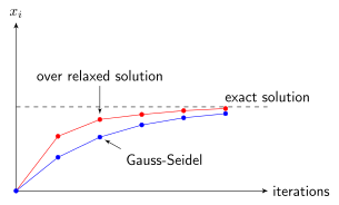
Fig. 7.4 Monotonic convergence of the Gauss-Seidel method. In this case choosing \(\omega>1\) may accelerate convergence.

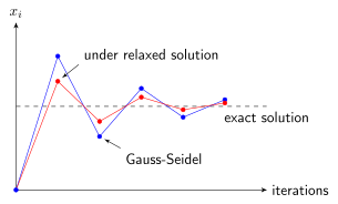
Fig. 7.5 Oscillatory convergence of the Gauss-Seidel method. In this case choosing \(\omega<1\) may reduce oscillations.

When the Gauss-Seidel iterates converge monotonically (Fig. 7.4), choosing \(\omega > 1\) often accelerates convergence. When the Gauss-Seidel iterates oscillate about the exact solution, (Fig. 7.5), choosing \(\omega < 1\) can dampen oscillations and improve convergence. For most practical problems, choosing \(\omega \ge 2\) causes the method to become unstable and divergence is likely. Consequently the relaxation parameter is usually restricted to \(0<\omega<2\).

Value of \(\omega\)	Interpretation
\(\omega = 1\)	Gauss-Seidel method
\(0 < \omega< 1\)	Under-relaxation
\(1 < \omega < 2\)	Over-relaxation
\(\omega \ge 2\)	Usually diverges

---

7.4.2. The iteration matrix for the SOR method

The convergence properties of the SOR method depend strongly on the choice of the relaxation parameter \(\omega\). Poor choices of \(\omega\) can lead to slower convergence than the Gauss-Seidel method or even divergence. As with the Jacobi and Gauss-Seidel methods, the convergence of the SOR method depends on the spectral radius of its iteration matrix. The method converges when

\[ \rho(T_{SOR}) < 1. \]

The iteration matrix for the SOR method is derived by writing the coefficient matrix of the linear system \(A\mathbf{x}=\mathbf{b}\) using

\[ A = L+\left(1-\frac{1}{\omega }\right)D+\frac{1}{\omega }D+U. \]

Substituting into the linear system \(A \mathbf{x} = \mathbf{b}\) and rearranging

\[\begin{split} \begin{align*} \left(L+\left(1-\frac{1}{\omega }\right)D+\frac{1}{\omega }D+U\right)\mathbf{x}&=\mathbf{b}\\ (D+\omega L)\mathbf{x}+((\omega -1)D+\omega U)\mathbf{x}&=\omega \mathbf{b}\\ (D+\omega L)\mathbf{x}&=((1-\omega )D-\omega U)\mathbf{x}+\omega \mathbf{b}\\ \mathbf{x}&=(D+\omega L)^{-1} ((1-\omega )D-\omega U)\mathbf{x}+(D+\omega L)^{-1} \omega \mathbf{b}. \end{align*} \end{split}\]

So the matrix form of the SOR method is

\[ \mathbf{x}^{(k+1)} =(D+\omega L)^{-1} ((1-\omega )D-\omega U)\mathbf{x}^{(k)} +(D+\omega L)^{-1} \omega \mathbf{b} \]

and the iteration matrix is

(7.10)\[ T_{SOR} =(D+\omega L)^{-1} ((1-\omega )D-\omega U). \]

The convergence properties of the SOR method depend on the choice of the relaxation parameter \(\omega\). Since the SOR method is based upon the Gauss-Seidel method, the diagonal dominance test for convergence also applies to the SOR method.

---

7.4.3. Optimum value of the relaxation parameter

The optimum value of \(\omega\) will be the one that minimises the spectral radius of the iteration matrix. The iteration matrix will depend on the value of \(\omega\). One way to estimate the optimum value of \(\omega\) is to calculate \(\rho(T_{SOR})\) for values in the range \(\omega \in [0, 2]\) and choose the value of \(\omega\) which minimises this value. This has been done for the system of linear equations from Example 7.1 and the plot is shown in Fig. 7.6.

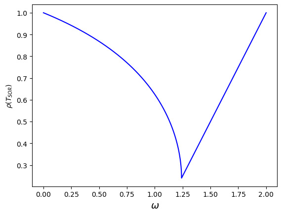
Fig. 7.6 Plot of the spectral radius \(\rho(T_{SOR})\) of the iteration matrix for the SOR method when used to solve the system of linear equations from Example 7.1.

The optimal relaxation parameter corresponds to the minimum point on the graph. At this value, the spectral radius is smallest and the error decreases most rapidly from one iteration to the next. An estimation of the optimum value of the relaxation parameter is \(\omega = 1.25\).

The optimal value of \(\omega\) depends on the coefficient matrix and is generally not known in advance. In practice it is often estimated experimentally or approximated using theoretical results. If the coefficient matrix \(A\) has real eigenvalues we can use the following theorem to calculate the exact value of \(\omega\).

Theorem 7.3 (Optimum relaxation parameter)

If the eigenvalues of the Jacobi iteration matrix \(T_J\)​ are real, then the optimum relaxation parameter is

(7.11)\[ \omega_{opt} = 1+{\left(\frac{\rho (T_J )}{1+\sqrt{1-\rho (T_J )^2 }}\right)}^2, \]

where \(\rho(T_J)\) is the spectral radius of the iteration matrix of the Jacobi method calculation using equation jacobi-method-iteration-matrix-equation.

Example 7.5

Determine the optimum relaxation parameter for the SOR method when applied to the system of linear equations from Example 7.1 using equation (7.11).

---

Solution

We saw in Example 7.3 that the spectral radius of the iteration matrix for the Jacobi method for this system is \(\rho(T_J )=0.7906\).

Using equation (7.11)

\[ \begin{align*} \omega = 1 + \left( \frac{0.7906}{1 + \sqrt{1 - 0.7906^2}} \right)^2 \approx 1.2404. \end{align*} \]

Example 7.6

Solve the system of linear equations from from Example 7.1 using the SOR method with \(\omega = 1.24\) and an accuracy tolerance of \(\text{tol} = 10^{-4}\)

\[\begin{split} \begin{align*} 4x_1 +3x_2 &=-2,\\ 3x_1 +4x_2 -x_3 &=-8,\\ -x_2 +4x_3 &=14. \end{align*} \end{split}\]

---

Solution

The SOR method for this system is

\[\begin{split} \begin{align*} x_{1}^{(k+1)} &= (1 - \omega) x_{1}^{(k)} + \frac{\omega}{4} \left( -2 - 3 x_{2}^{(k)} \right), \\ x_{2}^{(k+1)} &= (1 - \omega) x_{2}^{(k)} + \frac{\omega}{4} \left( -8 - 3 x_{1}^{(k+1)} + x_{3}^{(k)} \right), \\ x_{3}^{(k+1)} &= (1 - \omega) x_{3}^{(k)} + \frac{\omega}{4} \left( 14 + x_{2}^{(k+1)} \right). \end{align*} \end{split}\]

Using starting values of \(\mathbf{x} = \mathbf{0}\). Computing the first iteration

\[\begin{split} \begin{align*} x_{1}^{(1)} &= (1 - 1.24) (0) + \frac{1.24}{4} \left( -2 - 3 (0) \right) = -0.62, \\ x_{2}^{(1)} &= (1 - 1.24) (0) + \frac{1.24}{4} \left( -8 - 3 (-0.62) + 0 \right) = -1.9034, \\ x_{3}^{(1)} &= (1 - 1.24) (0) + \frac{1.24}{4} \left( 14 + (-1.9034) \right) = 3.749946. \end{align*} \end{split}\]

Compute the residual

\[\begin{split} \begin{align*} \mathbf{r}^{(1)} = \mathbf{b} - A \mathbf{x}^{(1)} = \begin{pmatrix} -2 \\ -8 \\ 14 \end{pmatrix} - \begin{pmatrix} 4 & 3 & 0 \\ 3 & 4 & -1 \\ 0 & -1 & 4 \end{pmatrix} \begin{pmatrix} -0.62 \\ -1.9034 \\ 3.749946 \end{pmatrix} = \begin{pmatrix} 6.1902 \\ 5.223546 \\ -2.903184 \end{pmatrix}. \end{align*} \end{split}\]

Since \(\| \mathbf{r}^{(1)} \|_\infty = 6.1902 > 10^{-4}\) we continue iterating. Computing the second iteration

\[\begin{split} \begin{align*} x_{1}^{(2)} &= (1 - 1.24) (-0.62) + \frac{1.24}{4} \left( -2 - 3 (-1.9034) \right) = 1.298962, \\ x_{2}^{(2)} &= (1 - 1.24) (-1.9034) + \frac{1.24}{4} \left( -8 - 3 (1.298962) + 3.749946 \right) = -2.068735, \\ x_{3}^{(2)} &= (1 - 1.24) (3.749946) + \frac{1.24}{4} \left( 14 + (-2.068735) \right) = 2.798705. \end{align*} \end{split}\]

Compute the residual

\[\begin{split} \begin{align*} \mathbf{r}^{(2)} = \mathbf{b} - A \mathbf{x}^{(2)} = \begin{pmatrix} -2 \\ -8 \\ 14 \end{pmatrix} - \begin{pmatrix} 4 & 3 & 0 \\ 3 & 4 & -1 \\ 0 & -1 & 4 \end{pmatrix} \begin{pmatrix} 1.298962 \\ -2.068735 \\ 2.798705 \end{pmatrix} = \begin{pmatrix} -0.989642 \\ -0.823239 \\ 0.736445 \end{pmatrix}. \end{align*} \end{split}\]

Since \(\| \mathbf{r}^{(2)} \|_\infty = 0.989642 > 10^{-4}\) we continue iterating.

The SOR method was iterated until \(\| \mathbf{r}^{(k)} \|_\infty < 10^{-4}\) and the iteration values are given in the table below. Note that the SOR method took 9 iterations to achieve convergence to \(\text{tol}=10^{-4}\) whereas the Jacobi method took 49 iterations and the Gauss-Seidel method took 19 iterations to achieve the same accuracy.

\(k\)	\(x_{1}^{(k)}\)	\(x_{2}^{(k)}\)	\(x_{3}^{(k)}\)	\(\| \mathbf{r}^{(k)} \|_\infty\)
0	0.000000	0.000000	0.000000	14.000000
1	-0.620000	-1.903400	3.749946	6.19e+00
2	1.298962	-2.068735	2.798705	9.90e-01
3	0.992173	-2.038626	3.036337	2.14e-01
4	1.037801	-2.014620	2.986747	1.07e-01
5	1.004524	-2.004807	3.001690	1.16e-02
6	1.003385	-2.001470	2.999139	9.13e-03
7	1.000555	-2.000430	3.000073	9.29e-04
8	1.000267	-2.000122	2.999944	7.01e-04
9	1.000050	-2.000034	3.000003	9.65e-05

The table below compares the number of iteration required for the Jacobi, Gauss-Seidel and SOR methods to achieve convergence when applied to the same linear system used in the examples.

Method	Iterations
Jacobi	49
Gauss-Seidel	20
SOR (\(\omega = 1.24\))	9

For this example, the SOR method reduces the iteration count by more than 80% compared to the Jacobi method and by more than 50% compared to the Gauss-Seidel method.