2. Chapter 2. Explicit Runge-Kutta Methods

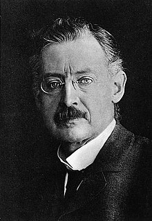
Fig. 2.1 Carl Runge (1856 - 1927)

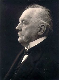
Fig. 2.2 Martin Kutta (1867 - 1944)

Fig. 2.3 Karl Heun (1859 - 1929)

The Runge-Kutta method is the most common numerical method used to solve ODEs. It was developed independently by German mathematicians Carl Runge and Martin Kutta in the late 19th century. The method involves approximating the solution of an ODE by computing the values of the solution at a series of discrete steps. At each step, the method uses a weighted average of the derivative of the solution at different points in the interval to estimate the value of the solution at the next time step. The method is iterative, meaning that the solution at each time step depends on the solution at the previous time step. Runge-Kutta methods are known as single step methods because to advance the solution to the next step we only require the values of the current step, as opposed to multistep methods such as the linear multistep methods family of methods that require values from multiple steps to compute the next step.

2.1. General form of a Runge-Kutta method

Definition 2.1 (General form of a Runge-Kutta method)

The general form of a Runge-Kutta method for solving the initial value problem \(y' =f(t,y)\), \(t \in [t_{\min}, t_{\max}]\), \(y_0 = y(t_{\min})\) is

(2.1)\[\begin{split} \begin{align} y_{n+1} &=y_n + h \sum_{i=1}^s b_i k_i,\\ k_i &= f(t_n +c_i h,y_n + h \sum_{j=1}^s a_{ij} k_j ), \end{align} \end{split}\]

where \(k_i\) for \(i = 1,2, \ldots, s\) are intermediate stage values used to calculate \(y_{n+1}\) and \(a_{ij}\), \(b_i\) and \(c_i\) are coefficients that define a particular Runge-Kutta method

For example, Huen’s method (also known as the modified Euler method) is a 2-stage Runge-Kutta method which is

(2.2)\[\begin{split} \begin{align*} y_{n+1} &= y_n + \frac{h}{2}(k_1 + k_2), \\ k_1 &= f(t_n, y_n), \\ k_2 &= f(t_n + h, y_n + h k_1), \\ \end{align*} \end{split}\]

The general form of a 2-stage method is

(2.3)\[\begin{split} \begin{align*} y_{n+1} &= y_n + h (b_1k_1 + b_2 k_2 ), \\ k_1 &= f(t_n + c_1 h, y_n + h(a_{11} k_1 + a_{12} k_2)), \\ k_2 &= f(t_n + c_2 h, y_n + h(a_{21} k_1 + a_{22} k_2)). \end{align*} \end{split}\]

So comparing equations (2.2) and (2.3) we can see that

\[\begin{split} \begin{align*} b_1 &= \tfrac{1}{2}, & b_2 &= \tfrac{1}{2}, & c_1 &= 0, & c_2 &= 1, \\ a_{11} &= 0, & a_{12} &= 0, & a_{21} &= 1, & a_{22} &= 0, \end{align*} \end{split}\]

2.1.1. Butcher tableau

Fig. 2.4 John Butcher

Runge-Kutta methods are often summarised in a Butcher tableau named after the New Zealand mathematician John Butcher.

Definition 2.2 (Butcher Tableau)

A Butcher tableau is a table of values containing the coefficients \(a_{ij}\), \(b_i\) and \(c_i\) for a Runge-Kutta method

\[\begin{split} \begin{align*} \begin{array}{c|cccc} c_1 & a_{11} & a_{12} & \cdots & a_{1s} \\ c_2 & a_{21} & a_{22} & \cdots & a_{2s} \\ \vdots & \vdots & \vdots & \ddots & \vdots \\ c_s & a_{s1} & a_{s2} & \cdots & a_{ss} \\ \hline & b_1 & b_2 & \cdots & b_s \end{array} \end{align*} \end{split}\]

For example, the Butcher tableau for Huen’s method (equation (2.2)) is

\[\begin{split} \begin{align*} \begin{array}{c|cccc} 0 & \\ 1 & 1 \\ \hline & 1/2 & 1/2 \end{array} \end{align*} \end{split}\]

Example 2.1

Write down the Butcher tableau for the 4-stage Runge-Kutta method given below as a Butcher tableau

\[\begin{split} \begin{align*} y_{n+1} &= y_n + \frac{h}{6}(k_1 + 2k_2 + 2k_3 + k_4), \\ k_1 &= f(t_n, y_n), \\ k_2 &= f(t_n + \tfrac{1}{2} h, y_n + \tfrac{1}{2} h k_1 ), \\ k_3 &= f(t_n + \tfrac{1}{2} h, y_n + \tfrac{1}{2} h k_2 ), \\ k_4 &= f(t_n + h, y_n + h k_3). \end{align*} \end{split}\]

Solution (click to show)

The general form of a 4-stage Runge-Kutta method is

\[\begin{split} \begin{align*} y_{n+1} &= y_n + h(b_1 k_1 + b_2 k_2 + b_3 k_3 + b_4 k_4), \\ k_1 &= f(t_n + c_1 h, y_n + h(a_{11}k_1 + a_{12}k_2 + a_{13}k_3 + a_{14}k_4)), \\ k_2 &= f(t_n + c_2 h, y_n + h(a_{21}k_1 + a_{22}k_2 + a_{23}k_3 + a_{24}k_4)), \\ k_3 &= f(t_n + c_3 h, y_n + h(a_{31}k_1 + a_{32}k_2 + a_{33}k_3 + a_{34}k_4)), \\ k_4 &= f(t_n + c_4 h, y_n + h(a_{41}k_1 + a_{42}k_2 + a_{43}k_3 + a_{44}k_4)). \end{align*} \end{split}\]

Comparing the Runge-Kutta method above to the general form of a 4-stage Runge-Kutta method we can see that the Butcher tableau is

\[\begin{split} \begin{align*} \begin{array}{c|cc} 0 & 0 & 0 & 0 & 0 \\ 1/2 & 1/2 & 0 & 0 & 0 \\ 1/2 & 0 & 1/2 & 0 & 0 \\ 1 & 0 & 0 & 1 & 0 \\ \hline & 1/6 & 1/3 & 1/3 & 1/6 \end{array} \end{align*} \end{split}\]

2.2. Explicit and implicit Runge-Kutta methods

The stage values for an \(s\)-stage Runge-Kutta method are

\[\begin{split} \begin{align*} k_1 &=f(t_n +c_1 h,y_n +h(a_{11} k_1 +a_{12} k_2 +\cdots +a_{1s} k_s )),\\ k_2 &=f(t_n +c_2 h,y_n +h(a_{21} k_1 +a_{22} k_2 +\cdots +a_{2s} k_s )),\\ &\vdots \\ k_s &=f(t_n +c_s h,y_n +h(a_{s1} k_1 +a_{s2} k_s +\cdots +a_{ss} k_s )). \end{align*} \end{split}\]

In the first equation we are calculating \(k_1\) includes \(k_1\) on the right-hand side and in the second equation we are calculating \(k_2\) includes \(k_2\) on the right-hand side and so on. These are examples of implicit functions and Runge-Kutta methods where the stage values are expressed using implicit functions are known as Implicit Runge-Kutta (IRK) methods. To calculate the solution of the stage values of an IRK method involves solving a system of equations (see Implicit Runge-Kutta Methods).

If the summation in the stage value \(k_i\) in equation (2.1) is altered so the upper limit to the sum is \(i-1\), i.e.,

\[ \begin{align*} k_i = f(t_n + c_i h,y_n + h\sum_{j=1}^{i-1} a_{ij} k_j) \end{align*} \]

and let \(c_1 = 0\) then we have the following equations for calculating the stage values

\[\begin{split} \begin{align*} k_1 &=f(t_n ,y_n),\\ k_2 &=f(t_n +c_2 h,y_n +ha_{21} k_1 ),\\ k_3 &=f(t_n +c_3 h,y_n +h(a_{31} k_1 +a_{32} k_2 )),\\ &\vdots \\ k_s &=f(t_n +c_s h,y_n +h(a_{s1} k_1 +a_{s2} k_s +\cdots +a_{s,s-1} k_{s-1} )). \end{align*} \end{split}\]

These stage values are explicit functions where the subject of the equation does not appear on the right-hand side. Runge-Kutta methods where the stages values are calculated using explicit functions are known as Explicit Runge Kutta (ERK) methods. These are easier to compute than implicit Runge-Kutta methods because the stage values can be calculated sequentially in order, i.e., \(k_1\) can be calculated using \(t_n\) and \(y_n\); \(k_1\) is then used to compute \(k_2\); \(k_1\) and \(k_2\) are then used to compute \(k_3\) and so on. However for some ODEs explicit methods require a very small value for the step length and and we must then use implicit methods (see the chapter on stability for more details).

2.2.1. Butcher tableau for explicit and implicit Runge-Kutta methods

Explicit and implicit Runge-Kutta methods can be easily distinguished by looking at their Butcher tableaux. The \(A\) matrix in the top right region of a Butcher tableau for an explicit method is lower-triangular (the values on the main diagonal and in the upper triangular region are all zeros) whereas for an implicit method the main-diagonal and upper triangular elements are non-zero.

Explicit Runge-Kutta method

\[\begin{split} \begin{array}{c|ccccc} 0 & 0 & & & & \\ c_2 & a_{21} & & & & \\ c_3 & a_{31} & a_{32} & & & \\ \vdots & \vdots & \vdots & \ddots & & \\ c_s & a_{s1} & a_{s2} & \cdots & a_{s,s-1} & \\ \hline & b_1 & b_2 & \cdots & b_{s-1} & b_s \end{array} \end{split}\]

Implicit Runge-Kutta method

\[\begin{split} \begin{array}{c|ccccc} c_1 & a_{11} & a_{12} & a_{13} & \cdots & a_{1s} \\ c_2 & a_{21} & a_{22} & a_{23} & \cdots & a_{2s} \\ c_3 & a_{31} & a_{32} & a_{33} & \cdots & a_{3s} \\ \vdots & \vdots & \vdots & \vdots & \ddots & \vdots \\ c_s & a_{s1} & a_{s2} & a_{s3} & \cdots & a_{ss} \\ \hline & b_1 & b_2 & b_3 & \cdots & b_s \end{array} \end{split}\]