4. Stability

The stability of a numerical solver for ordinary differential equations refers to its ability to produce accurate and reliable solutions over a long interval, without the computed values of the solution becoming unbounded or oscillatory. In other words, a stable numerical solver for ODEs is one that does not produce solutions that blow up or oscillate wildly as time goes on.

For example, consider the Euler method solution to the following initial value problem using step lengths of \(h = 0.25\) and \(h = 0.125\)

\[ y' = -15y, \qquad t \in [0, 1], \qquad y(0) = 1. \]

The exact solution for this initial value problem is \(y = e^{-15t}\) and the numerical solutions are plotted against the exact solution in Fig. 4.1. Here we can see that the solution using \(h = 0.125\) remains bounded whereas the solution using \(h = 0.25\) diverges.

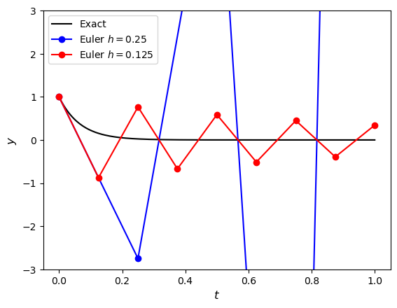
Fig. 4.1 Solutions to the initial value problem \(y' = -15y\), \(t\in [0, 1]\) and \(y(0) = 1\) using the Euler method with \(h=0.25\) and \(h=0.125\).

The solution using \(h = 0.125\) is an example of a stable solution where the numerical solution remains bounded whereas the solution using \(h = 0.25\) is an example of an unstable solution which is unbounded. The reason for the instability is due to the truncation of the Taylor series. We saw in the section on error analysis that the higher order terms that are omitted due to truncation causes a local truncation error, and the accumulation of these local truncation errors creates the global truncation error. If the local truncation error is too large then the global truncation error will eventually diverge as seen in Fig. 4.1 causing the solution to be unusable. This provides us with the definition of stability.

Definition 4.1 (Stability)

If \(e_n\) is the local truncation error of a numerical method defined by

\[\begin{align*} e_n = |y(t_{n}) - y_{n}|, \end{align*}\]

where \(y(t_n)\) is the exact solution and \(y_n\) the numerical approximation assuming that the solution at the previous step was exact. The method is considered stable if

(4.1)\[ |e_{n+1} - e_n | \leq 1, \]

for all steps of the method. If a method is not stable then it is unstable.

---

4.1. Stiffness

When solving IVPs numerically, some problems behave well and they can be solved accurately using large values of the step length \(h\). Other problems force us to use small step lengths use they become unstable. These problems as known as stiff problems.

An informal definition of stiffness is provided by Lambert [1991]

“If a numerical method with a finite region of absolute stability, applied to a system with any initial conditions, is forced to use in a certain interval of integration a step length which is excessively small in relation to the smoothness of the exact solution in that interval, then the system is said to be stiff in that interval.”

Given a linear system \(\mathbf{y}' = A \mathbf{y}\) then the stifness ratio is defined as

\[ S= \frac{\max_i (Re(\lambda_i))}{\min_i (Re(\lambda_i))},\]

where \(\lambda_i\) are the eigenvalues of the matrix \(A\). If the value of \(S\) is large, then the system is stiff. For example, consider the system

\[\begin{split} \begin{align*} y_1' &= -1000y_1 + 999y_2, \\ y_2' &= -y_2. \end{align*} \end{split}\]

Here \(A = \begin{pmatrix} -1000 & 999 \\ 0 & -1 \end{pmatrix}\), so the eigenvalues satisfy

\[\begin{split} \begin{align*} 0 &= | A - \lambda I | \\ &= \begin{vmatrix} -1000 - \lambda & 999 \\ 0 & -1 - \lambda \end{vmatrix} \\ &= (-1000-\lambda) (-1 - \lambda). \end{align*} \end{split}\]

So the eigenvalues are \(\lambda_1 = -1000\) and \(\lambda_2 =-1\) and the stiffness ratio is

\[ S = \frac{\lambda_1}{\lambda_2} = \frac{-1000}{-1} = 1000.\]

Since \(S\) is large then this is a stiff system.

A similar anaylsis can be performed for nonlinear systems using the Jacobian matrix to linearalise the system.

---

4.2. Stability functions

To examine the behaviour of the local truncation errors we use the following test equation

(4.2)\[ y' = \lambda y. \]

This test equation is chosen as it is a simple ODE which has the solution \(y=e^{\lambda t}\). Over a single step of a Runge-Kutta method, the values of \(y_{n+1}\) are updated using the values of \(y_n\), so the values of the local truncation error, \(e_{n+1}\), are also updated using \(e_n\) by the same method. This allows us to define a stability function for a method.

Definition 4.2 (Stability function)

The stability function of a method, denoted by \(R(z)\), is the rate of growth over a single step of the method when applied to calculate the solution of an ODE of the form \(y'=\lambda t\) where \(z = h \lambda\) and \(h\) is the step size

\[ y_{n+1} = R(z)y_n. \]

For example, if the Euler method is used to solve the test equation \(y'=\lambda y\) then the solution will be updated over one step using

\[ y_{n+1} = y_n + h f(t_n ,y_n) = y_n + h \lambda y_n, \]

Let \(z = h\lambda\) then

\[ y_{n+1} = y_n + z y_n =(1+z)y_n. \]

So the stability function of the Euler method is \(R(z) = 1 + z\).