2.6. Solving initial value problems using explicit Runge-Kutta methods

Recall that the general form of an explicit Runge-Kutta method is

\[\begin{split} \begin{align*} y_{n+1} &= y_n + h(b_1k_1 + b_2k_2 + \cdots + b_sk_s), \\ k_1 &= f(t_n, y_n), \\ k_2 &= f(t_n + c_2h, y_n + ha_{21}k_1), \\ k_3 &= f(t_n + c_3h, y_n + h(a_{31}k_1 + a_{32}k_2), \\ &\vdots \\ k_s &= f(t_n + c_sh, y_n + h(a_{s1}k_1 + a_{s2}k_2 + \cdots + a_{s,s-1}k_{s-1}). \end{align*} \end{split}\]

To apply the an explicit Runge-Kutta method to solve an initial value problem we calculate the stage values \(k_1, k_2, \dots, k_s\) using the known values of \(t_n\) and \(y_n\) and the step length \(h\). Then the solution over one step \(y_{n+1}\) is then calculated using \(k_1, k_2, \ldots, k_s\).

Algorithm 2.1 (Solving an IVP using an explicit Runge-Kutta method)

Inputs A first-order ODE of the form \(y' = f(t,y)\), a domain \(t \in [t_{\min}, t_{\max}]\), an initial value \(y(t_{\min})\) and a step length \(h\)

Outputs \(\vec{t}\) and \(\vec{y}\)

• \(\vec{t} \gets (t_{\min}, t_{\min} + h, t_{\min} + 2h, \ldots, t_{\max})\)

• \(\vec{y} \gets (y_0, 0, \ldots, 0)\)   (same size as \(\vec{t}\))

• For \(n = 0, \ldots, \operatorname{length}(\vec{t}) - 1\)

  • For \(i = 1, \ldots, s\)

    • \(k_i \gets f(t_n + c_i h, y_n + h (a_{i1}k_1 + a_{i2}k_2 + \cdots + a_{i,i-1}k_{i-1}))\)

  • \(y_{n+1} \gets y_n + h (b_1k_1 + b_2k_2 + \cdots + b_sk_s)\)

• Return \(\vec{t}, \vec{y}\)

Example 2.7

Calculate the solution to the following initial value problem using the RK4 method with \(h = 0.2\)

\[\begin{align*} y'=ty, \qquad t\in [0,1], \qquad y(0)=1. \end{align*}\]

Solution (click to show)

The RK4 method is

\[\begin{split} \begin{align*} y_{n+1} &= y_n + \frac{h}{6}(k_1 + 2k_2 + 2k_3 + k_4), \\ k_1 &= f(t_n, y_n), \\ k_2 &= f(t_n + \tfrac{1}{2}h, y_n + \tfrac{1}{2}hk_1), \\ k_3 &= f(t_n + \tfrac{1}{2}h, y_n + \tfrac{1}{2}hk_2), \\ k_4 &= f(t_n + h, y_n + hk_3). \end{align*} \end{split}\]

The values of \(t_n\) are

\[\begin{split} \vec{t} = \begin{pmatrix} 0.0 \\ 0.2 \\ 0.4 \\ 0.6 \\ 0.8 \\ 1.0 \end{pmatrix}. \end{split}\]

The ODE function is \(f(t, y) = ty\) and the initial value is \(y_0 = 1\). Calculating the stage values for the first step

\[\begin{split} \begin{align*} k_1 &= f(t_0, y_0) = t_0 y_0 \\ &= (0)(1) = 0, \\ k_2 &= f(t_0 + \tfrac{1}{2}h, y_0 + \tfrac{1}{2}hk_1) = (t_0 + \tfrac{1}{2}h)(y_0 + \tfrac{1}{2}hk_1) \\ &= (0 + \tfrac{1}{2}(0.2))(1 + \tfrac{1}{2}(0.2)(0)) = 0.1, \\ k_3 &= f(t_0 + \tfrac{1}{2}h, y_0 + \tfrac{1}{2}hk_2) = (t_0 + \tfrac{1}{2}h)(y_0 + \tfrac{1}{2}hk_2) \\ &= (0 + \tfrac{1}{2}(0.2))(1 + \tfrac{1}{2}(0.2)(0.1)) = 0.101, \\ k_4 &= f(t_0 + h, y_0 + hk_2) = (t_0 + h)(y_0 + hk_2) \\ &= (0 + 0.2)(1 + 0.2(0.1)) = 0.204. \end{align*} \end{split}\]

The solution at the first step is

\[\begin{split} \begin{align*} y_1 &= y_0 + \frac{h}{6}(k_1 + 2k_2 + 2k_3 + k_4) \\ &= 1 + \frac{0.2}{6}(0 + 2(0.1) + 2(0.101) + 0.204040) = 1.020201, \\ t_1 &= t_0 + h = 0 + 0.2 = 0.2 \end{align*} \end{split}\]

Repeating this for the other steps in the method gives the values in the table below.

\(n\)	\(t_n\)	\(y_n\)	\(k_1\)	\(k_2\)	\(k_3\)	\(k_4\)
0	0.0	1.000000	-	-	-	-
1	0.2	1.020201	0.000000	0.100000	0.101000	0.204040
2	0.4	1.083287	0.204040	0.312182	0.315426	0.433315
3	0.6	1.197217	0.433315	0.563309	0.569809	0.718349
4	0.8	1.377126	0.718330	0.888335	0.900235	1.101811
5	1.0	1.648717	1.101701	1.338567	1.359885	1.649103

2.6.1. Code

The code below defines a function called rk4() which computes the solution of an ODE over a single step. This can be used in the solveIVP() function (see the section on the Euler method).

Python

def rk4(f, t, y, h): 
    k1 = f(t, y)
    k2 = f(t + 0.5 * h, y + 0.5 * h * k1)
    k3 = f(t + 0.5 * h, y + 0.5 * h * k2)
    k4 = f(t + h, y + h * k3)
    return y + h / 6 * (k1 + 2 * k2 + 2 * k3 + k4)

MATLAB

function ynew = rk4(f, t, y, h)

k1 = f(t, y);
k2 = f(t + 0.5 * h, y + 0.5 * h * k1);
k3 = f(t + 0.5 * h, y + 0.5 * h * k2);
k4 = f(t + h, y + h * k3);
ynew = y + h / 6 * (k1 + 2 * k2 + 2 * k3 + k4);

end

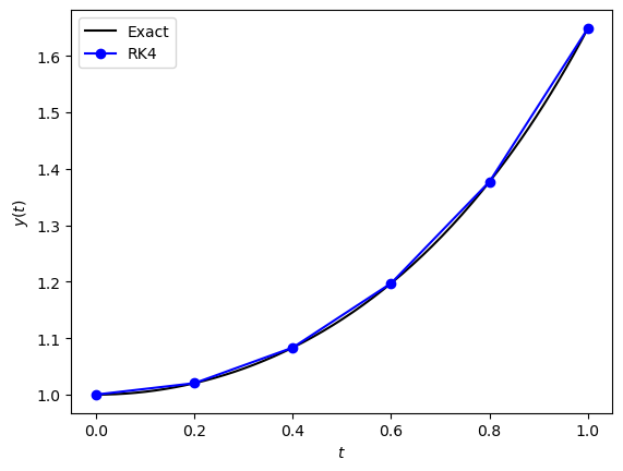
The rk4() function has been used to solve the IVP from Example 2.7 which is shown in Fig. 2.6.

Fig. 2.6 The solution to the IVP \(y'=ty\), \(t \in [0,1]\), \(y(0)=1\) using the RK4 method with \(h=0.2\).

2.6.2. Comparison of first, second and fourth-order solutions

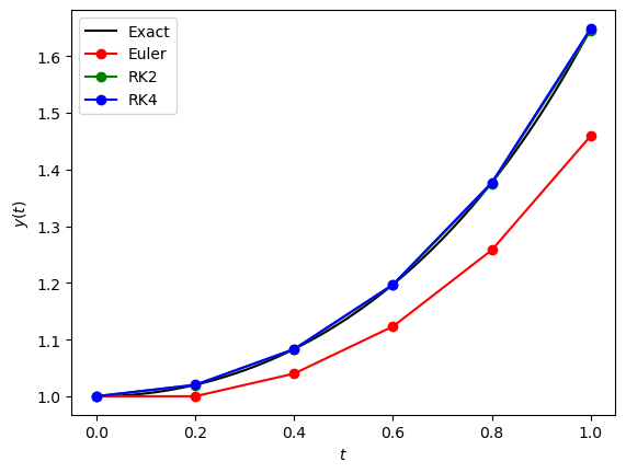
The first-order Euler method, the second-order Heun’s method and the fourth-order RK4 method solutions to the IVP from Example 2.7 have been plotted against the exact solution in Fig. 2.7.

Fig. 2.7 Comparisons between the Euler method, Heun’s method and the RK4 method for solving the IVP \(y'=ty\), \(t \in [0,1]\), \(y(0)=1\) with \(h=0.2\)

Here we see that the second-order and fourth-order method are significantly more accurate than the first-order method. However, in this plot it is difficult to see the difference between the second and fourth-order solutions.

We can compare the accuracy of different methods by computing the solutions for over different values of the step length and calculate the global truncation errors for a point in the domain. The three methods have been applied to solve the IVP from Example 2.7 using step lengths \(h = 0.2, 0.1, 0.05, 0.025\) and the global truncation error at \(t = 1\) has been calculated and shown in Table 2.2.

Table 2.2 Global truncation errors for the Euler method, Heun’s method and the RK4 method.

\(h\)	Euler (first-order)	Heun (second-order)	RK4 (fourth-order)
0.200	1.89e-01	3.88e-03	4.59e-06
0.100	1.02e-01	8.40e-04	2.64e-07
0.050	5.28e-02	1.92e-04	1.55e-08
0.025	2.69e-02	4.55e-05	9.33e-10

We have seen in chapter 1 that as the step lengths \(h\) decrease, the errors in the Euler method decrease in a linear fashion, i.e., \(E(h) = O(h)\), i.e., first-order accurate. We expect that Heun’s method and the RK4 method will have errors \(E(h) = O(h^2)\) and \(E(h) = O(h^4)\) respectively. By the definition of \(E(h) = O(h^n)\) the global truncation error should approximate \(E(h)=h^n\). Applying logarithms to both sides gives

\[ \begin{align*} \log(E(h)) &= n\log(h). \end{align*} \]

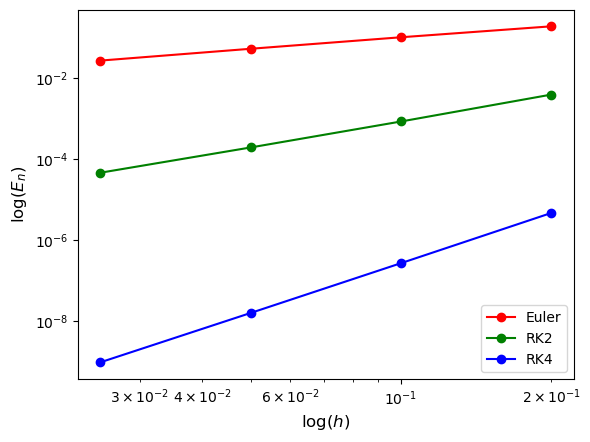
This is a linear function where the slope of \(\log(E(h))\) has a gradient of \(n\). The global truncation errors for the three methods have been plotted on a loglog scale in Fig. 2.8

Fig. 2.8 Plots of the the global truncation errors for the Euler method, Heuns’ method and the RK4 method on a loglog scale.

The loglog plots of the global truncation errors are linear functions where we can clearly see the distinction between the errors for the three methods. The order of the methods \(n\) can be approximated using

(2.17)\[ n \approx \frac{\log(E(h_1) - \log(E(h_2))}{\log(h_1) - \log(h_2)}, \]

where \(h_1 > h_2\). Using the values from Table 2.2

\[\begin{split} \begin{align*} \text{Euler}: && n & \approx \frac{\log(1.89\times 10^{-1}) - \log(2.69\times 10^{-2})}{\log(0.2) - \log(0.025)} = 0.94 \approx 1, \\ \text{Heun}: && n & \approx \frac{\log(3.88 \times 10^{-3}) - \log(4.55 \times 10^{-5})}{\log(0.2) - \log(0.025)} = 2.14 \approx 2, \\ \text{RK4}: && n & \approx \frac{\log(4.59 \times 10^{-6}) - \log(9.33 \times 10^{-10})}{\log(0.2) - \log(0.025)} = 4.09 \approx 4, \end{align*} \end{split}\]

which confirm the order of accuracy of the three methods.