5.3. The finite-difference method

The finite-difference method for solving a boundary value problem replaces the derivatives in the ODE with finite-difference approximations derived from the Taylor series. This results in linear system of algebraic equations that can be solved to give an approximation of the solution to the BVP.

The derivatives of \(y_i\) are approximated using values of neighbouring nodes \(y_{i+1}\), \(y_{i-1}\) etc. using expressions derived by truncating the Taylor series and rearranging to make the derivative term the subject. Some common finite-difference approximations are tabulated below.

Finite-difference approximation	Error	Name
\(y' = \dfrac{y_{i+1} - y_i}{h}\)	\(O(h)\)	Forward difference
\(y' = \dfrac{y_i - y_{i-1}}{h}\)	\(O(h)\)	Backward difference
\(y' = \dfrac{y_{i+1} - y_{i-1}}{2h}\)	\(O(h^2)\)	Central difference
\(y'' = \dfrac{y_{i-1} - 2 y_i + y_{i+1}}{h^2}\)	\(O(h^2)\)	Symmetric difference

The solution to a boundary value problem using then finite-difference method is determined by approximating the derivatives in the ODE using finite-differences. Consider the following boundary value problem

\[ \begin{align*} y'' = f(t,y), \qquad t \in [t_0, t_{\max}], \qquad y(t_0) = a, \qquad y(t_{\max}) = b. \end{align*} \]

Using the symmetric difference to approximate \(y''\) in the ODE we have

\[\begin{split} \begin{align*} \frac{y_{i-1} - 2y_i + y_{i+1}}{h^2} &= f(t_i ,y_i) \\ y_{i-1} - 2y_i + y_{i+1} &= h^2f(t_i, y_i). \end{align*} \end{split}\]

Since we know that \(y_0 = a\) and \(y_n = b\) then

\[\begin{split} \begin{align*} y_0 &= a, \\ y_0 - 2y_1 + y_2 &= h^2 f(t_1, y_1), \\ y_1 - 2y_2 + y_3 &= h^2 f(t_2, y_2), \\ & \vdots \\ y_{n-3} - 2y_{n-2} + y_{n-1} &= h^2 f(t_{n-2}, y_{n-2}), \\ y_{n-2} - 2y_{n-1} + y_{n} &= h^2 f(t_{n-1}, y_{n-1}), \\ y_{n} &= b, \end{align*} \end{split}\]

which can be written as the matrix equation

\[\begin{split} \begin{align*} \begin{pmatrix} 1 & 0 \\ 1 & -2 & 1 \\ & 1 & -2 & 1 \\ & & \ddots & \ddots & \ddots \\ & & & 1 & -2 & 1 \\ & & & & 1 & -2 & 1 \\ & & & & & 0 & 1 \end{pmatrix} \begin{pmatrix} y_0 \\ y_1 \\ y_2 \\ \vdots \\ y_{n-2} \\ y_{n-1} \\ y_n \end{pmatrix} = \begin{pmatrix} a \\ f(t_1, y_1) \\ f(t_2, y_2) \\ \vdots \\ f(t_{n-2}, y_{n-2} \\ f(t_{n-1}, y_{n-1}) \\ b \end{pmatrix}. \end{align*} \end{split}\]

Example 5.4

Use the finite-difference method to solve the boundary below using a step length of \(h = 0.2\)

\[ \begin{align*} y'' - y' - y = 0, \qquad y(0) = 0, \qquad y(1) = 2. \end{align*} \]

---

Solution

Using a forward difference to approximate \(y'\) and a symmetric difference to approximate \(y''\) we have

\[ \begin{align*} \frac{y_{i-1} -2y_i +y_{i+1} }{h^2 }-\frac{y_{i+1} -y_i }{h}-y_i = 0, \end{align*} \]

which can be simplified to

\[ \begin{align*} y_{i-1} +(h-h^2 -2)y_i +(1-h)y_{i+1} = 0. \end{align*} \]

This gives the following system of linear equations

\[\begin{split} \begin{align*} y_0 &= 0, \\ y_0 + (h - h^2 - 2) y_1 + (1 - h) y_2 &= 0, \\ y_1 + (h - h^2 - 2) y_2 + (1 - h) y_3 &= 0, \\ &\vdots \\ y_{n-3} + (h - h^2 - 2) y_{n-2} + (1 - h) y_n &= 0, \\ y_{n-2} + (h - h^2 - 2) y_{n-1} + (1 - h) y_n &= 0, \\ y_n &= 2. \end{align*} \end{split}\]

which we can write the linear system as the matrix equation

\[\begin{split} \begin{align*} \begin{pmatrix} 1 & 0 & & & & \\ 1 & h-h^2 -2 & 1-h & & & \\ & \ddots & \ddots & \ddots & \\ & & 1 & h-h^2 -2 & 1-h \\ & & & 0 & 1 \end{pmatrix} \begin{pmatrix} y_0 \\ y_1 \\ \vdots \\ y_{n-1} \\ y_n \end{pmatrix} = \begin{pmatrix} 0 \\ 0 \\ \vdots \\ 0 \\ 2 \end{pmatrix}. \end{align*} \end{split}\]

If we use a step length of \(h=0.2\) we have

\[ \begin{align*} \vec{t} = (0, 0.2, 0.4, 0.6, 0.8, 1), \end{align*} \]

and

\[\begin{split} \begin{align*} \begin{pmatrix} 1 & 0 \\ 1 & -1.84 & 0.8 \\ & 1 & -1.84 & 0.8 \\ & & 1 & -1.84 & 0.8 \\ & & & 1 & -1.84 & 0.8 \\ & & & & 0 & 1 \end{pmatrix} \begin{pmatrix} y_0 \\ y_1 \\ y_2 \\ y_3 \\ y_4 \\ y_5 \end{pmatrix} = \begin{pmatrix} 0 \\ 0 \\ 0 \\ 0 \\ 0 \\ 2 \end{pmatrix}. \end{align*} \end{split}\]

Solving this system of linear equations gives

\[ \mathbf{y} = (0, 0.2060, 0.4738, 0.8322, 1.3219, 2). \]

---

5.3.1. Code

The code below calculates the solution to the boundary value problem in Example 5.4.

Python

import numpy as np
import matplotlib.pyplot as plt

# Define BVP parameters
tspan = [0, 1]          # boundaries of the t domain
bvals = [0, 2]          # boundary values
h = 0.2                 # step length

# Define linear system
n = int((tspan[1] - tspan[0]) / h) + 1
t = np.arange(n) * h    # t array
A = np.eye(n)
b = np.zeros(n)
b[0], b[-1] = bvals[0], bvals[1]
for i in range(1, n-1):
    A[i,i-1] = 1
    A[i,i] = h - h ** 2 - 2
    A[i,i+1] = 1 - h
        
# Solve linear system
y = np.linalg.solve(A, b)

MATLAB

% Define BVP parameters
tspan = [0, 1];
bvals = [0, 2];
h = 0.2;

% Define linear system
n = floor((tspan(2) - tspan(1)) / h) + 1;
t = (tspan(1) : h : tspan(2));
A = eye(n);
b = zeros(n, 1);
b(1) = bvals(1);
b(n) = bvals(2);
for i = 2 : n - 1
    A(i, i-1) = 1;
    A(i, i) = h - h ^ 2 - 2;
    A(i, i+1) = 1 - h;
end

% Solve linear system
y = A \ b;

5.3.2. Order vs number of nodes

The solutions seen in Example 5.4 seem to show that the finite-difference method produces reasonably accurate results for this boundary value problem. One way to improve on the accuracy of our solution is to increase the number of nodes used.

Consider the solution of the following BVP using the finite-difference method

\[ y'' + 3ty' + 7y = \cos (2t), \qquad y(0) = 1, \qquad y(3) = 0. \]

Using forward and symmetric differences to approximate \(y'\) and \(y''\) respectively gives

\[\begin{split} \begin{align*} \frac{y_{i-1} - 2y_i + y_{i+1}}{h^2} + 3t_i \left( \frac{y_{i+1} - y_i}{h}\right) + 7y_i &= \cos(2t_i) \\ y_{i-1} + (7h^2 - 3ht_i - 2)y_i + (1 + 3ht_i)y_{i+1} &= h^2 \cos(2t_i). \end{align*} \end{split}\]

So the linear system is

\[\begin{split} \begin{align*} \begin{pmatrix} 1 & 0 \\ 1 & 7h^2 - 3ht_1 - 2 & 1 + 3ht_1 \\ & \ddots & \ddots & \ddots \\ && 1 & 7h^2 - 3ht_{N-1} - 2 & 1 + 3ht_{N-1} \\ &&& 0 & 1 \end{pmatrix} \begin{pmatrix} y_0 \\ y_1 \\ \vdots \\ y_{N-1} \\ y_N \end{pmatrix} \\ = \begin{pmatrix} 1 \\ h^2 \cos(2t_1) \\ \vdots \\ h^2 \cos(2t_{N-1}) \\ 0 \end{pmatrix}. \end{align*} \end{split}\]

The solution of this BVP is shown in Fig. 5.4 for \(h=0.05\) and \(h = 0.005\). Since we used a first-order approximation for \(y'\) the error for this method is \(O(h)\) and we expect the solution using \(h=0.005\) to be more accurate.

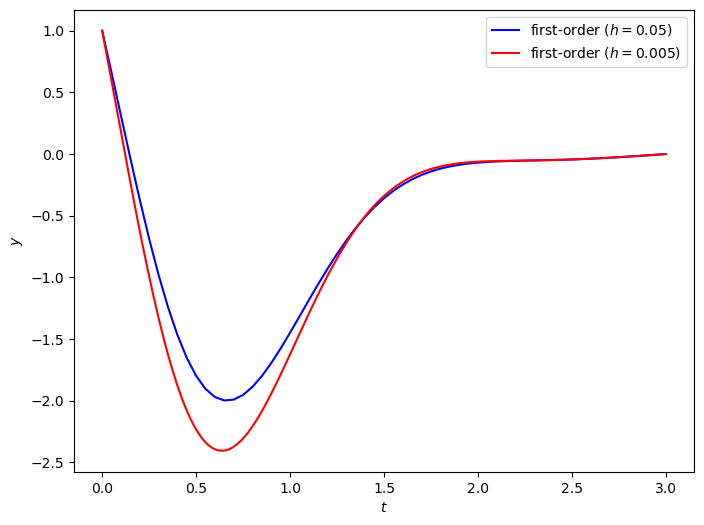
Fig. 5.4 Solutions to the boundary value problem \(y'' + 3ty' + 7y = \cos (2t)\), \(t \in [0,3]\), \(y(0) = 1\), \(y(3) = 0\) using first-order finite-difference approximations with \(h=0.05\) and \(h=0.005\).

To obtain a more accurate solution, instead of increasing the number of nodes we could use the central difference approximation (which is second-order accurate) to approximate \(y'\)

\[\begin{split} \begin{align*} \frac{y_{i-1} - 2y_i + y_{i+1}}{h^2} + 3t_i\left( \frac{y_{i+1} - y_{i-1}}{2h} \right) + 7y_i &= \cos(2t_i) \\ (2 - 3ht_i)y_{i-1} + (14h^2 - 4)y_i + (2 + 3ht_i)y_{i+1} &= 2h^2 \cos(2t_i). \end{align*} \end{split}\]

So the linear system for the second-order finite-difference method is

\[\begin{split} \begin{align*} \begin{pmatrix} 1 & 0 \\ 2 - 3ht_1 & 14h^2 - 4 & 2 + 3ht_1 \\ & \ddots & \ddots & \ddots \\ && 2 - 3ht_{N-1} & 14h^2 - 4 & 2 + 3ht_{N-1} \\ &&& 0 & 1 \end{pmatrix} \begin{pmatrix} y_0 \\ y_1 \\ \vdots \\ y_{N-1} \\ y_N \end{pmatrix} \\ = \begin{pmatrix} 1 \\ 2h^2 \cos(2t_1) \\ \vdots \\ 2h^2 \cos(2t_{N-1}) \\ 0 \end{pmatrix}. \end{align*} \end{split}\]

The solution using the second-order finite difference method with \(h=0.05\) has been plotted against the first-order solution using \(h=0.05\) and \(h=0.005\) in Fig. 5.5. The second order solution gives good agreement with the first order solution using 10 times fewer nodes.

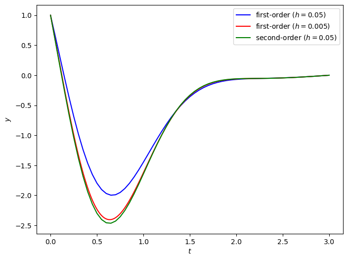
Fig. 5.5 Solutions to the boundary value problem \(y'' + 3ty' + 7y = \cos (2t)\), \(t \in [0,3]\), \(y(0) = 1\), \(y(3) = 0\) using first-order and second-order finite-difference approximations with \(h=0.05\) and \(h=0.005\).