2.8. Explicit Runge-Kutta Methods Exercises

Exercise 2.1

Write the following Runge-Kutta method in a Butcher tableau.

\[\begin{align*} y_{n+1} &=y_n +\frac{h}{6}(k_1 +4k_3 +k_4 ),\\ k_1 &=f(t_n ,y_n ),\\ k_2 &=f(t_n +\frac{1}{4}h,y_n +\frac{1}{4}hk_1 ),\\ k_3 &=f(t_n +\frac{1}{2}h,y_n +\frac{1}{2}hk_2 ),\\ k_4 &=f(t_n +h,y_n +h(k_1 -2k_2 +2k_3 )). \end{align*}\]

Solution

\[\begin{split} \begin{array}{c|cccc} 0 & 0 \\ \frac{1}{4} & \frac{1}{4} \\ \frac{1}{2} & 0 & \frac{1}{2} \\ 1 & 1 & -2 & 2 \\ \hline & \frac{1}{6} & 0 & \frac{2}{3} & \frac{1}{6} \end{array} \end{split}\]

Exercise 2.2

Write out the equations for the following Runge-Kutta method.

\[\begin{align*}\begin{array}{c|cccc} 0 & & & & \\ \frac{1}{4} & \frac{1}{4} & & & \\ \frac{1}{2} & -\frac{1}{2} & 1 & & \\ 1 & \frac{1}{4} & 0 & \frac{3}{4} & \\ \hline & 0 & \frac{4}{9} & \frac{1}{3} & \frac{2}{9} \end{array}\end{align*}\]

Solution

\[\begin{split} \begin{align*} y_{n+1} &= y_n + \frac{h}{9} (4k_2 + 3k_3 + 2k_4), \\ k_1 &= f(t_n, y_n), \\ k_2 &= f(t_n + \tfrac{1}{4}h, y_n + \tfrac{1}{4}h k_1), \\ k_3 &= f(t_n + \tfrac{1}{2}h, y_n + h(-\tfrac{1}{2}k_1 + k_2)), \\ k_4 &= f(t_n + h, y_n + h(\tfrac{1}{4}k_1 + \tfrac{3}{4}k_3)). \end{align*} \end{split}\]

Exercise 2.3

Derive an explicit second-order Runge-Kutta method where \(b_1 =\frac{1}{3}\). Express your solution as Butcher tableau.

Solution

\[\begin{split} \begin{array}{c|cc} 0 & 0 \\ \frac{3}{4} & \frac{3}{4} & 0 \\ \hline & \frac{1}{3} & \frac{2}{3} \end{array} \end{split}\]

Exercise 2.4

Determine the order, elementary weight and density of this rooted tree.

Solution

\[\begin{split} \begin{align*} r(\tau) &= 10, \\ \Phi(\tau) &= \sum_{i,j,k,\ell} b_i a_{ij} a_{ik} a_{k\ell} c_j^3 c_k c_\ell^2, \\ \gamma(\tau) &= 600. \end{align*} \end{split}\]

Exercise 2.5

Derive the order conditions for a third-order explicit Runge-Kutta method.

Solution

\[\begin{split} \begin{align*} b_1 + b_2 + b_3 &= 1, \\ b_2 c_2 + b_3 c_3 &= \frac{1}{2}, \\ b_2 c_2^2 + b_3 c_3^2 &= \frac{1}{3}, \\ b_3 a_{32} c_2 &= \frac{1}{6}, \\ a_{21} &= c_2, \\ a_{31} + a_{32} &= c_3. \end{align*} \end{split}\]

Exercise 2.6

Derive an explicit fourth-order Runge-Kutta method where \(c_2 = \frac{1}{3}\), \(c_3 = \frac{1}{2}\) and \(c_4 = 1\). Express your method in using a Butcher tableau.

Hint: you might not need all of the row-sum conditions to get a solution.

Solution

\[\begin{split} \begin{array}{c|cccc} 0 & 0 \\ \frac{1}{3} & \frac{1}{3} \\ \frac{1}{2} & \frac{1}{8} & \frac{3}{8} \\ 1 & \frac{1}{2} & -\frac{3}{2} & 2 \\ \hline & \frac{1}{6} & 0 & \frac{2}{3} & \frac{1}{6} \end{array} \end{split}\]

Exercise 2.7

Using pen and paper, apply your Runge-Kutta method derived in Exercise 2.3 to solve the following initial value problem using a step length of \(h=0.4\)

\[\begin{align*} y' = t - y, \qquad t\in [0,2],\qquad y(0)=1 \end{align*}\]

Write your solutions correct to 4 decimal places.

Solution

\(t_n\)	\(y_n\)	\(k_1\)	\(k_2\)
0.00	1.0000	-	-
0.40	0.7600	-1.0000	-0.4000
0.80	0.7248	-0.3600	0.0480
1.20	0.8289	0.0752	0.3526
1.60	1.0276	0.3711	0.5598
2.00	1.2908	0.5724	0.7007

Exercise 2.8

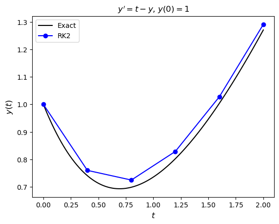
Write a Python of MATLAB program that computes the solution to the IVP from Exercise 2.7 using the second-order ERK method derived in Exercise 2.3. The exact solution to this IVP is \(y = t + 2e^{-t} - 1\), produce a plot of the solution and the exact solution on the same set of axes.

Solution

Exercise 2.9

A third-order explicit Runge-Kutta method has the Butcher tableau

\[\begin{split} \begin{array}{c|ccc} 0 & 0 \\ \frac{1}{2} & \frac{1}{2} \\ 1 & -1 & 2 \\ \hline & \frac{1}{6} & \frac{2}{3} & \frac{1}{6} \end{array} \end{split}\]

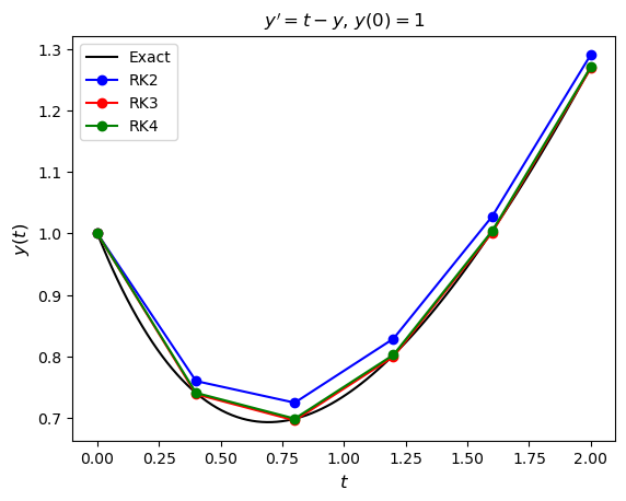
Write a Python or MATLAB program which uses this third-order method, and the fourth-order method derived in Exercise 2.6, to solve the IVP from Exercise 2.7. Produce a plot the compares the second-, third- and fourth-order solutions to the exact solution.

Solution

Exercise 2.10

Repeat the calculations from Exercise 2.9 using a range of values of the step length starting at \(h=0.4\) and halving each time until \(h = 0.025\).

(a)   Calculate the global truncation error for \(y(2)\) for each of the solutions and present this information in a table

(b)   Product a plot of the global truncation errors against \(h\) for each of the ERK methods using logarithmic scales for the horizontal and vertical axes.

(c)   Use the global truncation errors to estimate the order of the ERK methods.

Hint: you can use the NumPy command idx = np.argmin(abs(t - 2)) or the MATLAB command [~,idx] = min(abs(t - 2)) to determine the index of the value in the array t which is closest to 2.

Solution

(a)

|   h   |   RK2    |   RK3    |   RK4    |
|:-----:|:--------:|:--------:|:--------:|
| 0.400 | 2.01e-02 | 1.99e-03 | 1.61e-04 | 
| 0.200 | 4.23e-03 | 2.12e-04 | 8.53e-06 | 
| 0.100 | 9.74e-04 | 2.44e-05 | 4.90e-07 | 
| 0.050 | 2.34e-04 | 2.93e-06 | 2.94e-08 | 
| 0.025 | 5.75e-05 | 3.60e-07 | 1.80e-09 | 

(b)

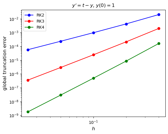
(c)   RK2: \(n \approx 2.11\), RK3: \(n \approx 3.11\), RK4: \(n \approx 4.11\)

Exercise 2.11

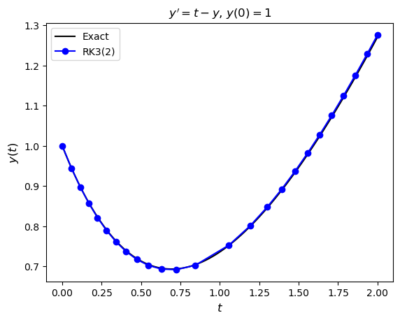
Combining Heun’s method and Kutta’s third-order method gives the following Butcher tableau for an embedded Runge-Kutta method

\[\begin{split} \begin{array}{c|ccc} 0 & \\ \frac{1}{2} & \frac{1}{2} \\ 1 & -1 & 2 \\ \hline & \frac{1}{6} & \frac{2}{3} & \frac{1}{6} \\ & 0 & 1 & 0 \end{array}\end{split}\]

where the first row of the \(b\) coefficients gives the third-order accurate solution and the second row gives the second-order accurate solution. Write a Python or MATLAB program that solves the initial value problem from Exercise 2.7 using an absolute tolerance of \(10^{-6}\) and a relative tolerance of \(10^{-3}\).

(a)   Produce a plot that compares the numerical solution with the exact solution.

Solution

(b)   Determine the number of successful steps, failed steps and the number of times the ODE function was evaluated.

Solution

There were 24 successful steps, 2 failed steps and 78 function evaluations.