3.4. Implicit Runge-Kutta methods exercises#
Exercise 3.1
Determine the order of the DIRK method shown below.
Solution
This DIRK method is a second-order method.
Exercise 3.2
Derive a third-order Radau IIA method. Present your method in a Butcher tableau.
Solution
Exercise 3.3
Consider following IVP
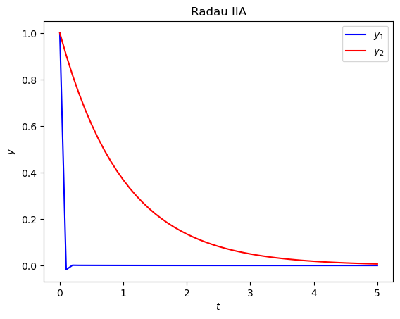
(a) Compute the solution to this IVP over \(t\in [0, 5]\) using the Radau IIA method from the previous exercise with a step length of \(h = 0.1\). Produce a plot of the solutions to \(y_1\) and \(y_2\) against \(t\).
Solution
(b) Attempt to solve this IVP using the RK4 method with the same step length. What do you notice about the result?
Solution
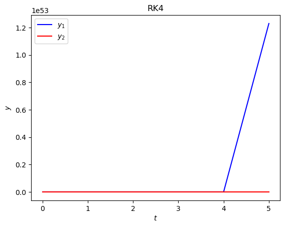
The solution is unstable.
(c) Solve this IVP using the Fehlberg 4(5) explicit Runge-Kutta method. Record the time taken for both methods to compute the solution and determine value of the smallest step length used in the Fehlberg’s method solution. What does this suggest about this system?
Solution
The Radau IIA method took 0.005 seconds to compute whereas the Runge-Kutta Fehlberg 4(5) method took 0.051 seconds to compute (these times will vary depending on the machine used). The smallest step length used in Fehlberg’s method was \(h = 0.000427\). This suggests that this is a stiff system since the minimum step length used in Fehlberg’s method is very small compared to the one used for the Radau IIA method.
3.4.1. Solutions#
The solutions to these exercises downloaded below by right clicking on the link and select ‘Save Link As’: