1.4. Higher-order ODEs

The Euler method solves a first-order ODE of the form \(y' = f(t, y)\), so what happens when we want to solve a higher order ODE? The solution is we write a higher order ODE as system of first-order ODEs and apply the Euler method to solve the system. For example consider the \(N\)-th order ODE

\[ y^{(N)} = f(t, y, y', y'' ,\ldots ,y^{(N-1)}). \]

If we introduce functions \(y_1, y_2, \ldots, y_N\) where \(y_1=y\), \(y_2 =y'\), \(y_3 =y''\) and so on then

\[\begin{split} \begin{align*} y_1' &= y_2,\\ y_2' &= y_3,\\ &\vdots \\ y_N' &= f(t, y_1 , y_2 , y_3 , \ldots, y_{N-1}). \end{align*} \end{split}\]

This is a system of \(N\) first-order ODEs, so we can apply the Euler method to solve the system to give an equivalent solution to the \(N\)-th order ODE.

Example 1.3

A mass-spring-damper model consists of objects connected via springs and dampers. A simple example of the application of a model is a single object connected to a surface is shown in Fig. 1.10.

Fig. 1.10 The mass-spring-damper model [Wikipedia, 2008].

The displacement of the object over time can be modelled by the second-order ODE

\[ m \ddot{y} + c \dot{y} + k y = 0, \]

where \(y\) represents the displacement of e object, \(\dot{y}\) represents the change in the displacement over time (i.e., velocity), \(m\) represents the mass of the object, \(c\) is the damping coefficient and \(k\) is a spring constant based on the length and elasticity of the spring.

An object of mass 1kg is connected to a dampened spring with \(c = 2\) and \(k = 4\). The object is displaced by 1m and then released. Use the Euler method to compute the displacement of the object over the first 5 seconds after it was released.

Solution (click to show)

We first need to rewrite the governing equation as a system of first-order ODEs. Let \(y_1 = y\) and \(y_2 = \dot{y}\) then we have the system of two first-order ODEs

\[\begin{split} \begin{align*} \dot{y}_1 &= y_2, \\ \dot{y}_2 &= \frac{1}{m}(- c y_2 - k y_1). \end{align*} \end{split}\]

Since \(m = 1\), \(c = 2\) and \(k = 4\) then writing the system in vector form \(\dot{\mathbf{y}} = \mathbf{f}(t, \mathbf{y})\) gives

\[\begin{split} \begin{align*} \mathbf{y} &= (y_1, y_2), \\ \mathbf{f}(t, \mathbf{y}) &= (y_2, \quad -2y_2 - 4y_1). \end{align*} \end{split}\]

The initial conditions are \(y_1 = 1\) (displacement) and \(y_2 = 0\) (velocity of the object). Using the Euler method with a step length of \(h = 0.1\)

\[\begin{split} \begin{align*} \mathbf{y}_1 &= \mathbf{y}_0 + h \mathbf{f}(t_0, \mathbf{y}_0), \\ &= (1, 0) + 0.1 (0, \quad -2(0) - 4(1)) \\ &= (1, -0.04), \\ t_1 &= t_0 + h = 0 + 0.1 = 0.1, \\ \\ \mathbf{y}_2 &= \mathbf{y}_1 + h \mathbf{f}(t_1, \mathbf{y}_1), \\ &= (1, -0.04) + 0.1 (-0.04, \quad -2(-0.04) - 4(1)) \\ &= (0.96, -0.72), \\ t_2 &= t_1 + h = 0.1 + 0.1 = 0.2, \\ \\ \mathbf{y}_3 &= \mathbf{y}_2 + h \mathbf{f}(t_2, \mathbf{y}_2), \\ &= (0.96, -0.72) + 0.1 (-0.72, \quad -2(-0.72) - 4(0.96)) \\ &= (0.888, -0.96), \\ t_3 &= t_2 + h = 0.2 + 0.1 = 0.3, \\ & \vdots \end{align*} \end{split}\]

A plot of the displacement of the object in the first 5 seconds of being released is shown in

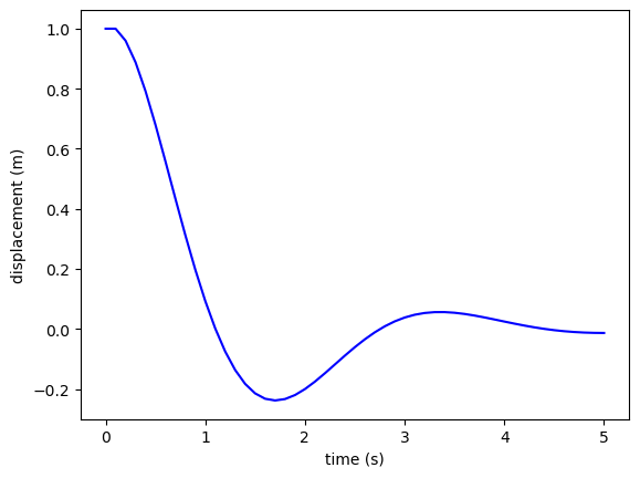
Fig. 1.11 Euler method solutions for the mass-spring-damper model with \(m = 1\), \(c = 2\), \(k = 4\) and initial displacement 1m.

1.4.1. Code

The code below sets up and solves the mass-sprint-damper model example from Example 1.3 using the Euler method.

Python

# Define mass-spring-damper model
def spring(t, y):
    return np.array([ y[1], (- c * y[1] - k * y[0]) / m ])
    

# Define IVP parameters
tspan = [0, 5]  # boundaries of the t domain
y0 = [1, 0]     # initial values
h = 0.1         # step length
m = 1;          # mass of object
c = 2;          # damping coefficient
k = 4;          # spring constant

# Solve the IVP using the Euler method
t, y = euler(spring, tspan, y0, h)
print(y)

# Plot solution
fig, ax = plt.subplots()
plt.plot(t, y[:,0], "b-")
plt.xlabel("time (s)", fontsize=12)
plt.ylabel("displacement (m)", fontsize=12)
plt.show()

MATLAB

% Define mass-spring-damper model
spring = @(t, y, m, c, k) [ y(2), (-c * y(2) - k * y(1)) / m];

% Define IVP parameters
tspan = [0, 5];  % boundaries of the t domain
y0 = [1, 0];     % initial values [S, I, R]
h = 0.1;         % step length
m = 1;           % mass of object
c = 2;           % damping coefficient
k = 4;           % spring constant

% Solve the IVP using the Euler method
[t, y] = euler(@(t, y)spring(t, y, m, c, k), tspan, y0, h);

% Plot solution
plot(t, y(:, 1), 'b-', LineWidth=2)
xlabel('time (s)', Fontsize=14, Interpreter='latex')
ylabel('displacement (m)', Fontsize=14, Interpreter='latex')
axis padded