7.2. The Gauss-Seidel method#

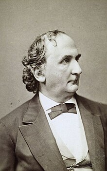
Fig. 7.2 Carl Friedrich Gauss (1777 - 1855)#
In the previous section we saw that the Jacobi method for solving a linear system \(A \mathbf{x} = \mathbf{b}\) computes a new estimate of the solution based on the current estimates. So when computing the new approximation \(x_i^{(k+1)}\), all other variables are taken from iteration \(k\), even if improved values have already been computed during the current iteration.
The key idea behind the Gauss-Seidel method, named after German mathematicians Carl Gauss and Philipp von Seidel, is that once a new approximation has been computed, it is used immediately in subsequent calculations. This means that each iteration uses more up-to-date information than the Jacobi method.
The Jacobi method is
Since \(x_1^{(k+1)}, \ldots, x_{i-1}^{(k+1)}\) have already been computed, then the Gauss-Seidel method is
Definition 7.3 (The Gauss-Seidel method)
The Gauss-Seidel method for solving a system of linear equations of the form \(A \mathbf{x} = \mathbf{b}\) is
where \(a_{ii} \ne 0\).
Example 7.2
Compute the solution to the system of linear equations from Example 7.1 (shown below) using the Gauss-Seidel method with an accuracy tolerance of \(\text{tol} = 10^{-4}\)
Solution
The Gauss-Seidel method for this system is
Using starting values of \(\mathbf{x} = \mathbf{0}\). Computing the first iteration
Compute the residual
Since \(\| \mathbf{r}^{(1)} \|_\infty = 4.875 > 10^{-4}\) we continue iterating. Computing the second iteration
Compute the residual
Since \(\| \mathbf{r}^{(2)} \|_\infty = 0.421875 > 10^{-4}\) we continue iterating.
The Gauss-Seidel method was iterated until \(\|\mathbf{r}\|_\infty < 10^{-4}\) and a selection of the iteration values are given in the table below. Note that the Gauss-Seidel method took 20 iterations to achieve convergence to \(\text{tol}=10^{-4}\) whereas the Jacobi method took 49 iterations to achieve the same accuracy.
\(k\) |
\(x_{1}^{(k)}\) |
\(x_{2}^{(k)}\) |
\(x_{3}^{(k)}\) |
\(\| \mathbf{r} \|_\infty\) |
|---|---|---|---|---|
0 |
0.000000 |
0.000000 |
0.000000 |
14.000000 |
1 |
-0.500000 |
-1.625000 |
3.093750 |
4.88e+00 |
2 |
0.718750 |
-1.765625 |
3.058594 |
4.22e-01 |
3 |
0.824219 |
-1.853516 |
3.036621 |
2.64e-01 |
4 |
0.890137 |
-1.908447 |
3.022888 |
1.65e-01 |
5 |
0.931335 |
-1.942780 |
3.014305 |
1.03e-01 |
\(\vdots\) |
\(\vdots\) |
\(\vdots\) |
\(\vdots\) |
|
19 |
0.999905 |
-1.999921 |
3.000020 |
1.43e-04 |
20 |
0.999940 |
-1.999950 |
3.000012 |
8.93e-05 |
7.2.1. Code#
The code below defines the function gauss_seidel() which solves a linear system of equations of the for \(A \mathbf{x} = \mathbf{b}\) using the Gauss-Seidel method.
def gauss_seidel(A, b, tol=1e-6):
    n = len(b)
    x = np.zeros(n)
    maxiter = 100
    for k in range(maxiter):
        for i in range(n):
            sum_ = 0
            for j in range(n):
                if i != j:
                    sum_ += A[i,j] * x[j]

            x[i] = (b[i] - sum_) / A[i,i]

        r = b - np.dot(A, x)

        if max(abs(r)) < tol:
            break

    return x
function x = gauss_seidel(A, b, tol)

n = length(b);
x = zeros(n, 1);
maxiter = 100;
for k = 1 : 100
    for i = 1 : n
        sum_ = 0;
        for j = 1 : n
            if j ~= i
                sum_ = sum_ + A(i,j) * x(j);
            end
        end
        x(i) = (b(i) - sum_) / A(i,i);
    end
    r = b - A * x;
    if max(abs(r)) < tol
        break
    end
end

end