3.3. Solving initial value problems using implicit Runge-Kutta methods

Recall that the general form of a Runge-Kutta method is

(3.1)\[\begin{split} \begin{align*} y_{n+1} &= y_n + h \sum_{i=1}^s b_i k_i,\\ k_i &= f(t_n +c_i h,y_n + h \sum_{j=1}^s a_{ij} k_j). \end{align*} \end{split}\]

To simplify the calculations for implicit methods we introduce a variable \(Y_i\), such that

(3.2)\[Y_i = y_n + h \displaystyle\sum_{j=1}^s a_{ij} k_j, \]

so the stage values are

\[ \begin{align*} k_i = f(t_n + c_i h, Y_i). \end{align*} \]

Substituting \(k_i\) into the expressions \(y_{n+1}\) from equation (3.1)

(3.3)\[ \begin{align*} y_{n+1} &= y_n + h \sum_{i=1}^s b_i f(t_n + c_i h, Y_i). \end{align*} \]

Also, substituting the expression for \(k_j\) into equation (3.2) gives an implicit expression for \(Y_i\)

(3.4)\[ Y_i = y_n + h \sum_{j=1}^s a_{ij} f(t_n + c_i h, Y_j). \]

In doing this we have simplified the stage value calculations \(k_i\) so that the ODE function \(f(t, y)\) is calculated using a single value \(Y_i\) as opposed to a summation of multiple \(k_i\) values. Once the values of \(Y_i\) are found we then apply equation (3.3) to advance the solution by one step.

---

3.3.1. Solving for \(Y_i\)

The values of \(Y_i\) are found by solving a system of equations. In practice the solution of this system of equations is done using Newton’s method with the derivatives approximated using finite-difference approximations. This can be quite an involved process and is outside the scope of these notes, so we shall be solving these systems either using an iterative method.

The idea behind an iterative method to solve a system of equations is that we start with a guess of the solution and use this guess value to compute an improved guess value. We continue to do this until the difference between two successive guess values is sufficiently small, and we are satisfied that our guess is close enough to the solution of the linear system.

Let \(Y_i^{(k)}\) denote the \(k\)-th guess value for \(Y_i\) then using equation (3.4) the iterative equations are

\[ \begin{align*} Y_i^{(k+1)} &= y_n + h\sum_{j=1}^s a_{ij} f(t_n + c_i, Y_j^{(k)}). \end{align*} \]

If \(tol\) is an tolerance for the desired accuracy then we cease iterations when

\[ \max_i( |Y_i^{(k+1)} - Y_i^{(k)}|) < tol.\]

This iterative method is a form of the Gauss-Seidel method which we will be using to solve systems of linear equations in Chapter 7. The psuedocode for solving an IVP using an IRK method with the \(Y_i\) calculated using an iterative method is shown below.

Algorithm 3.1 (Solving an IVP using an implicit Runge-Kutta method)

Inputs A first-order ODE of the form \(y' = f(t,y)\), a domain \(t \in [t_0, t_{\max}]\), an initial value \(y(t_0) = y_0\) and a step length \(h\)

Outputs \((t_0, t_1, \ldots)\) and \((y_0, y_1, \ldots)\)

• \(nsteps \gets \operatorname{int}\left( \dfrac{b - a}{h} \right)\)

• \(Y_i \gets 1\) and \(Y_i^{(old)} \gets 1\) for all \(i = 1, \ldots, s\)

• For \(n = 0, \ldots, nsteps\)

  • For \(k = 1, \ldots, 100\)

    • \(Y_i \gets y_n + h \displaystyle\sum_{j = 1}^s f(t_n + c_i h, Y_i)\) for all \(i = 1, \ldots, s\)

    • If \(\max_i(|Y_i - Y_i^{(old)}|) < tol\)

      • Exit \(k\) loop

    • \(Y_i^{(old)} \gets Y_i\) for all \(i = 1, \ldots, s\)

  • \(y_{n+1} \gets y_n + h (b_1k_1 + b_2k_2 + \cdots + b_sk_s)\)

  • \(t_{n+1} \gets t_n + h\)

• Return \((t_0, t_1, \ldots)\) and \((y_0, y_1, \ldots)\)

Example 3.5

The third-order Radau IA implicit Runge-Kutta method is defined by the following Butcher tableau

\[\begin{align*} \begin{array}{c|cc} 0 & 1/4 & -1/4 \\ 2/3 & 1/4 & 5/12 \\ \hline & 1/4 & 3/4 \end{array} \end{align*}\]

Use this method to calculate the solution of the following initial value problem using a step length of \(h=0.2\) and a convergence tolerance of \(tol=10^{-4}\).

\[\begin{align*} y' = ty, \qquad t\in [0,1], \qquad y(0)=1. \end{align*}\]

Solution (click to show)

The \(Y_i\) values for this method are

\[\begin{split} \begin{align*} Y_1 &= y_n + h(\tfrac{1}{4}f(t_n + 0h, Y_1) - \tfrac{1}{4}f(t_n + \tfrac{2}{3}h, Y_2)), \\ Y_2 &= y_n + h(\tfrac{1}{4}f(t_n + 0h, Y_1) + \tfrac{5}{12}f(t_n + \tfrac{2}{3}h, Y_2)). \end{align*} \end{split}\]

Since \(f(t,y) = ty\) then

\[\begin{split} \begin{align*} Y_1 &= y_n + h(\tfrac{1}{4}t_nY_1 - \tfrac{1}{4}(t_n+\tfrac{2}{3}h)Y_2), \\ Y_2 &= y_n + h(\tfrac{1}{4}t_nY_1 + \tfrac{5}{12}(t_n+\tfrac{2}{3}h)Y_2). \end{align*} \end{split}\]

so the iterative equations are

\[\begin{split} \begin{align*} Y_1^{(k+1)} &= y_n + h(\tfrac{1}{4}t_nY_1^{(k)} - \tfrac{1}{4}(t_n+\tfrac{2}{3}h)Y_2^{(k)}), \\ Y_2^{(k+1)} &= y_n + h(\tfrac{1}{4}t_nY_1^{(k)} + \tfrac{5}{12}(t_n+\tfrac{2}{3}h)Y_2^{(k)}). \end{align*} \end{split}\]

Using starting guess values of \(Y_1^{(0)} = Y_2^{(0)} = 1\) (these are arbitrary but must be non-zero) then

\[\begin{split} \begin{align*} Y_1^{(1)} &= 1 + 0.2(\tfrac{1}{4}(0)(1) - \tfrac{1}{4}(0+\tfrac{2}{3}(0.2))(1)) = 0.993333, \\ Y_2^{(1)} &= 1 + 0.2(\tfrac{1}{4}(0)(1) + \tfrac{5}{12}(0+\tfrac{2}{3}(0.2))(1)) = 1.011111. \end{align*} \end{split}\]

The maximum difference between \(Y_i^{(1)}\) and \(Y_i^{(0)}\) is

\[\begin{split} \begin{align*} \max(| Y_1^{(1)} - Y_1^{(0)}|, |Y_2^{(1)} - Y_2^{(0)}|) &= \max(| 0.003333 - 1|, |1.011111 - 1|) \\ &= 0.01111, \end{align*} \end{split}\]

since \(0.01111 > 10^{-4}\) the guess values \(Y_i^{(1)}\) do not satisfy the accuracy requirement. Repeating the calculations we have the values given in the table below.

| \(k\) | \(Y_1^{(k)}\) | \(Y_2^{(2)}\) | \(\max_i (|Y_i^{(k)} - Y_i^{(k-1)}|)\) | |:—:|:———–:|:———–:|:————–:| | 0 | 1 | 1 | - | | 1 | 0.993333 | 1.011111 | 1.11e-2 | | 2 | 0.993259 | 1.011235 | 1.23e-4 | | 3 | 0.993258 | 1.011236 | 1.37e-6 |

It took 3 iterations to reached the desired accuracy where \(Y_1 = 0.993258\) and \(Y_2 = 1.011236\). Using these values we can calculate the solution over the first step

\[\begin{split} \begin{align*} y_1 &= y_0 + h(\tfrac{1}{4}f(t_0, Y_1) + \tfrac{3}{4}f(t_0 + \tfrac{2}{3}h, Y_2) \\ &= 1 + 0.2(\tfrac{1}{4}(0)(0.993258) + \tfrac{3}{4}(0 + \tfrac{2}{3}(0.2), 1.011236)) \\ &= 1.020225. \end{align*} \end{split}\]

The solution to this initial value problem using the Radau IA method is shown in the table below along with the values of \(Y_1\) and \(Y_2\) and the number of iterations required to achieve the desired accuracy.

\(n\)	\(t_n\)	\(y_n\)	\(Y_1\)	\(Y_2\)	Iterations
0	0.0	1.000000	-	-	-
1	0.2	1.020225	0.993258	1.011236	3
2	0.4	1.083341	1.012690	1.059789	3
3	0.6	1.197317	1.073989	1.156207	4
4	0.8	1.377300	1.184716	1.313100	4
5	1.0	1.649006	1.359225	1.552411	5

3.3.2. Code

The code below defines a function called radauIA() which computes the solution to an initial value problem using the Radau IA method. The stage values are contained in Y1 and Y2 and the previous values are contained in Y1old and Y2old. Iterations continue until the maximum difference between the new and previous values are less than \(10^{-4}\) or when 10 iterations have been completed, whichever comes first.

Python

def radauIA(f, tspan, y0, h, tol=1e-4):
    
    # Calculate number of steps required
    nsteps = int((tspan[1] - tspan[0]) / h)

    # Initialise t and y arrays
    t = np.zeros(nsteps + 1)
    y = np.zeros((nsteps + 1, len(y0)))
    t[0] = tspan[0]
    y[0,:] = y0

    # Initialise Y1 and Y2 arrays
    Y1, Y2 = np.ones(len(y0)), np.ones(len(y0))
    Y1old, Y2old = Y1, Y2

    # Loop through the steps
    for n in range(nsteps):

        # Solve for Y1 and Y2
        for k in range(10):
            Y1 = y[n,:] + h * (1/4 * f(t[n], Y1) - 1/4 * f(t[n] + 2/3 * h, Y2))
            Y2 = y[n,:] + h * (1/4 * f(t[n], Y1) + 5/12 * f(t[n] + 2/3 * h, Y2))

            if max(np.amax(abs(Y1 - Y1old)), np.amax(abs(Y2 - Y2old))) < tol:
                break

            Y1old, Y2old = Y1, Y2

        # Update solution
        y[n+1,:] = y[n,:] + h * (1/4 * f(t[n], Y1) + 3/4 * f(t[n] + 2/3 * h, Y2))
        t[n+1] = t[n] + h

    return t, y

MATLAB

function ynew = radauIA(f, t, y, h)

neq = length(y);
Y1 = ones(neq);
Y2 = ones(neq);
Y1old = ones(neq);
Y2old = ones(neq);
for k = 1 : 10
    Y1 = y + h * (1/4 * f(t, Y1) - 1/4 * f(t + 2/3 * h, Y2));
    Y2 = y + h * (1/4 * f(t, Y1) + 5/12 * f(t + 2/3 * h, Y2));
    if max(max(abs(Y1 - Y1old)), max(abs(Y2 - Y2old))) < 1e-4
        break
    end
    Y1old = Y1;
    Y2old = Y2;
end
ynew = y + h / 4 * (f(t, Y1) + 3 * f(t + 2/3 * h, Y2));

end

The radauIA() function has been used to plot the solutions to the IVP from Example 3.5 which is shown in Fig. 3.1,

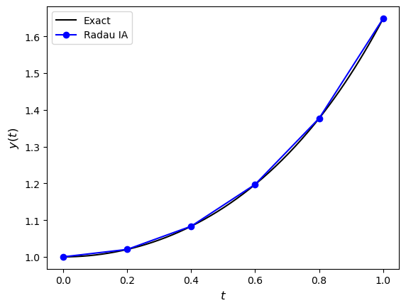
Fig. 3.1 The solution to the IVP \(y'=ty\), \(t \in [0,1]\), \(y(0)=1\) using the RadauIA method with \(h=0.2\) and \(tol=10^{-4}\).