4.4. Stability functions of implicit methods

The simplest implicit method for solving ODEs is the implicit Euler method (also known as the backward Euler method) which is

\[ y_{n+1} =y_n + hf(t_{n+1}, y_{n+1}). \]

Applying this to solve the test equation \(y' = \lambda y\) and rearranging gives

\[\begin{split} \begin{align*} y_{n+1} &=y_n + h \lambda y_{n+1} \\ (1 - h\lambda ) y_{n+1} &=y_n \\ y_{n+1} &=\left( \frac{1}{1 - h\lambda} \right) y_n. \end{align*} \end{split}\]

Let \(z = h\lambda\) then the stability function for the implicit Euler method is

\[ R(z)=\frac{1}{1-z}. \]

So here the stability function is a ration fraction which is the case for all implicit methods so we write

\[ R(z) = \frac{P(z)}{Q(z)}. \]

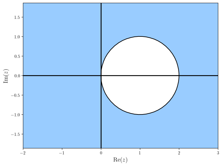
The region of absolute stability of the implicit Euler method has been plotted in Fig. 4.6. Note that the region of absolute stability includes all of the complex plane with the exception of the unshaded region which means the interval of absolute stability is \(h\lambda \in [-\infty, 0]\) so the method is stable for all values of \(h\) when solving the test equation \(y'= \lambda y\) (this is known as A-stability).

Fig. 4.6 Region of absolute stability for the implicit Euler method.

4.4.1. Stability functions for an implicit Runge-Kutta method

To determine the stability function for an implicit Runge-Kutta method we consider the stability function of a general Runge-Kutta method given in equations (4.3) and (4.4) which are repeated below

\[\begin{split} \begin{align*} y_{n+1} & = y_n + z \vec{b}^\mathrm{T} Y, \\ Y &= \vec{e} y_n + z A Y. \end{align*} \end{split}\]

Rewriting these gives

\[\begin{split} \begin{align*} y_{n+1} - z \vec{b}^\mathrm{T} Y &= y_n \\ (I - z A) Y &= \vec{e}y_n. \end{align*} \end{split}\]

We can write these as a matrix equation

\[\begin{split} \begin{align*} \begin{pmatrix} 1 & -z b_1 & -z b_2 & \cdots & -z b_s \\ 0 & 1-z a_{11} & -z a_{12} & \cdots & -z a_{1s} \\ 0 & -z a_{21} & 1-z a_{22} & \cdots & -z a_{2s} \\ \vdots & \vdots & \vdots & \ddots & \vdots \\ 0 & -z a_{s1} & -z a_{s2} & \cdots & 1-z a_{ss} \end{pmatrix} \begin{pmatrix} y_{n+1} \\ Y_1 \\ Y_2 \\ \vdots \\ Y_s \end{pmatrix}= \begin{pmatrix} y_n \\ y_n \\ y_n \\ \vdots \\ y_n \end{pmatrix}. \end{align*} \end{split}\]

Using Cramer’s rule to solve this system for \(y_{n+1}\) we have

\[\begin{split} \begin{align*} y_{n+1} = \frac{\det \begin{pmatrix} y_n & -zb_1 & -zb_2 & \cdots & -zb_s \\ y_n & 1-za_{11} & -za_{12} & \cdots & -za_{1s} \\ y_n & -za_{21} & 1-za_{22} & \cdots & -za_{2s} \\ \vdots & \vdots & \vdots & \ddots & \vdots \\ y_n & -za_{s1} & -za_{s2} & \cdots & 1-za_{ss} \end{pmatrix}}{\det (I-zA)}. \end{align*} \end{split}\]

Performing a row operation of subtracting the first row of matrix from all other rows gives

\[\begin{split} \begin{align*} y_{n+1} =\frac{\det \begin{pmatrix} y_n & -zb_1 & -zb_2 & \cdots & -zb_s \\ 0 & 1-za_{11} +zb_1 & -za_{12} +zb_2 & \cdots & -za_{1s} +zb_s \\ 0 & -za_{21} +zb_1 & 1-za_{22} +zb_2 & \cdots & -za_{2s} +zb_s \\ \vdots & \vdots & \vdots & \ddots & \vdots \\ 0 & -za_{s1} +zb_1 & -za_{s2} +zb_2 & \cdots & 1-za_{ss} +zb_s \end{pmatrix}}{\det(I-zA)}. \end{align*} \end{split}\]

This provides the following definition of the stability function for an implicit Runge-Kutta method.

Definition 4.8 (Stability function of an implicit Runge-Kutta method)

The stability function of an implicit Runge-Kutta method is

(4.7)\[R(z) = \frac{\det (I - zA + z\vec{e}\vec{b}^\mathrm{T})}{\det(I - zA)}.\]

where \(\vec{e}\vec{b}^\mathrm{T}\) is a diagonal matrix with the elements of \(\vec{b}\) on the main diagonal

\[\begin{split} \begin{align*} \vec{e}\vec{b}^\mathrm{T} = \begin{pmatrix} b_1 & 0 & \cdots & 0 \\ 0 & b_2 & \ddots & \vdots \\ \vdots & \ddots & \ddots & 0 \\ 0 & \cdots & 0 & b_s \end{pmatrix}. \end{align*} \end{split}\]

4.4.2. A-stability

If we compare the plot of the regions of absolute stability for the explicit Euler method (Fig. 4.3) and that of the implicit Euler method (Fig. 4.6) we can see that the implicit method has a much greater stability region than explicit method. This also applies to other implicit methods and as such are very useful for solving stiff ODEs where the stability constraints placed on an explicit method means the step length \(h\) is too small to be of practical use. A desirable property of some implicit methods is that there is no limit placed on the value of \(h\) for which will result in an unstable method, this is known as A-stability.

Definition 4.9 (A-stability)

A method is said to be A-stable if its region of absolute stability satisfies

\[ \{ z : z \in {\mathbb{C}}^- ,|R(z)| \leq 1\} \]

i.e., the method is stable for all points in the left-hand side of the complex plane.

Theorem 4.1 (Conditions for A-stability)

Given an implicit Runge-Kutta method with a stability function of the form

\[ R(z) = \frac{P(z)}{Q(z)} \]

and define the \(E\)-polynomial function

(4.8)\[ E(y)=Q(iy)Q(-iy)-P(iy)P(-iy), \]

then the method is A-stable if and only if the following are satisfied

• All roots of \(Q(z)\) have positive real parts;

• \(E(y)\geq 0\) for all \(y\in \mathbb{R}\).

Example 4.3

An implicit Runge-Kutta method is defined by the following Butcher tableau

\[\begin{split} \begin{align*} \begin{array}{c|cc} 1/3 & 5/12 & -1/12 \\ 1 & 3/4 & 1/4 \\ \hline & 3/4 & 1/4 \end{array} \end{align*} \end{split}\]

Determine whether this method is A-stable and plot the region of absolute stability.

Solution (click to show)

Using equation (4.7)

\[\begin{split} \begin{align*} R(z) &= \frac{\det \left( \begin{pmatrix} 1 & 0 \\ 0 & 1 \end{pmatrix} - z \begin{pmatrix} 5/12 & -1/12 \\ 3/4 & 1/4 \end{pmatrix} + z \begin{pmatrix} 3/4 & 0 \\ 0 & 1/4 \end{pmatrix} \right)}{\det \left( \begin{pmatrix} 1 & 0 \\ 0 & 1 \end{pmatrix} - z \begin{pmatrix} 5/12 & -1/12 \\ 3/4 & 1/4 \end{pmatrix} \right)} \\ &= \frac{\det \begin{pmatrix} 1 + z/3 & z/12 \\ -3z/4 & 1 \end{pmatrix}} {\det \begin{pmatrix} 1 - 5z/12 & z/12 \\ -3z/4 & 1 - z/4 \end{pmatrix}} = \frac{1 + \frac{1}{3}z + \frac{1}{16}z^2}{1 - \frac{2}{3}z + \frac{1}{6}z^2}. \end{align*} \end{split}\]

Here \(Q(z) = 1 - \frac{2}{3}z + \frac{1}{6}z^2\) which has roots at \(z = 2 \pm \sqrt{2}\) which both have positive real parts so the first condition for A-stability is satisfied. Using equation (4.8)

\[\begin{split} \begin{align*} E(y) &= \left( 1 - \frac{2}{3} i y - \frac{1}{6}y^2 \right) \left( 1 + \frac{2}{3} i y - \frac{1}{6}y^2 \right) \\ & \qquad - \left( 1 + \frac{1}{3} i y - \frac{1}{16} y^2 \right) \left( 1 - \frac{1}{3}i y - \frac{1}{16}y^2 \right) \\ &= \left( 1 + \frac{2}{3}iy - \frac{1}{6}y^2 - \frac{2}{3} i y + \frac{4}{9}y^2 + \frac{1}{9} i y^3 - \frac{1}{6}y^2 - \frac{1}{9} i y^2 + \frac{1}{36} y^4 \right) \\ & \qquad \left( 1 - \frac{1}{3} i y - \frac{1}{16}y^2 + \frac{1}{3} i y + \frac{1}{9} y^2 - \frac{1}{48} i y^2 - \frac{1}{16} y^2 + \frac{1}{48} i y^3 + \frac{1}{256} y^4 \right) \\ &= \left( 1 + \frac{1}{9} y^2 + \frac{1}{36} y^4 \right) - \left( 1 - \frac{1}{72} y^2 + \frac{1}{256} y^4 \right) \\ &= \frac{1}{8} y^2 + \frac{55}{2304} y^4. \end{align*} \end{split}\]

Since \(y_2\) and \(y_4\) are positive for all \(y\) then \(E(y)>0\) and the second condition for A-stability is satisfied. Since both conditions are satisfied then we can say that this is an A-stable method.

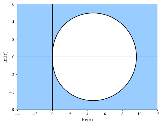
The region of absolute stability for this method has been plotted below. Note that the interval of absolute stability is \([-\infty, 0]\).

Code

Python

Determine stability function and check for A-stability.

import sympy as sp

# Define numerator and denominator functions
def P(z):
    return (I - z * A + z * ebT).det()

def Q(z):
    return (I - z * A).det()


# Define IRK method
A = sp.Matrix([[sp.Rational(5,12), -sp.Rational(1,12)],
            [sp.Rational(3,4), sp.Rational(1,4)]])
ebT = sp.Matrix([[sp.Rational(3,4), 0], [0, sp.Rational(1,4)]])
I = sp.eye(2)

# Calculate R(z)
z, y = sp.symbols('z, y')
R = P(z) / Q(z)
print(f"R(z) = ")
display(R)

# Check roots of Q have positive real parts
roots = sp.solve(Q(z) - 0)
print(f"Roots of Q(z)")
display(roots)

# Check E(y) >= 0
E = Q(1j * y) * Q(-1j * y) - P(1j * y) * P(-1j * y)
print(f"E(y) = ")
display(sp.simplify(sp.nsimplify(E)))

Plot the region of absolute stability.

import numpy as np
import matplotlib.pyplot as plt
plt.rcParams['text.usetex'] = True  # allows use of LaTeX in labels

# Generate Z values
xmin, xmax, ymin, ymax = -4, 12, -6, 6
X, Y = np.meshgrid(np.linspace(xmin, xmax, 200),np.linspace(ymin, ymax, 200))
Z = X + Y * 1j

# Define stability function
R = (1/16 * Z ** 2 + 1/3 * Z + 1) / (1/6 * Z ** 2 - 2/3 * Z + 1)

# Plot stability region
fig = plt.figure()
contour = plt.contourf(X, Y, abs(R), levels=[0, 1], colors="#99ccff")  # Plot stability region
plt.contour(X, Y, abs(R), colors= "k", levels=[0, 1])                  # Add outline
plt.axhline(0, color="k", linewidth=1)                                 # Add x-axis line
plt.axvline(0, color="k", linewidth=1)                                 # Add y-axis line
plt.axis("equal")
plt.axis([xmin, xmax, ymin, ymax])
plt.xlabel("$\mathrm{Re}(z)$", fontsize=12)
plt.ylabel("$\mathrm{Im}(z)$", fontsize=12)
plt.show()

MATLAB

Determine the stability function and check for A-stability.

% Define IRK method
A = [5/12, -1/12 ; 3/4, 1/4];
ebT = [3/4, 0 ; 0, 1/4];
I = eye(size(A, 1));

% Define numerator and denominator functions
P = @(z) det(I - z * A + z * ebT);
Q = @(z) det(I - z * A);

% Calculate R(z)
syms z y
Rz = P(z) / Q(z)

% Check roots of Q have positive real parts
roots_of_Q = solve(Q(z) == 0)

% Check E(y) >= 0
E = Q(1i * y) * Q(-1i * y) - P(1i * y) * P(-1i * y);
E = simplify(E)

Plot the region of absolute stability.

% Generate z values
xmin = -4;
xmax = 12;
ymin = -6;
ymax = 6;
[X, Y] = meshgrid(linspace(xmin, xmax, 200), linspace(ymin, ymax, 200));
Z = X + Y * 1i;

% Define stability function 
R = (1 + 1/3 * Z + 1/16 * Z .^ 2) ./ (1 - 2/3 * Z + 1/6 * Z .^ 2);

% Plot stability region
contourf(X, Y, abs(R), [0, 1], LineWidth=2)
xline(0, LineWidth=2)
yline(0, LineWidth=2)
colormap([153, 204, 255 ; 255, 255, 255] / 255)
axis equal
axis([xmin, xmax, ymin, ymax])
xlabel("$\mathrm{Re}(z)$", FontSize=12, Interpreter="latex")
ylabel("$\mathrm{Im}(z)$", FontSize=12, Interpreter="latex")