4.3. Stability function of a Runge-Kutta method

Recall that the general form of a Runge-Kutta method is

\[\begin{split} \begin{align*} y_{n+1}&=y_n + h \sum_{i=1}^s b_i k_i ,\\ k_i &=f(t_n +c_i h,y_n +h\sum_{j=1}^s a_{ij} k_j ). \end{align*} \end{split}\]

Let \(Y_i = y_n + h \displaystyle \sum_{j=1}^s a_{ij} k_i\) and applying the method to the test equation \(y' = \lambda y\) we have

\[\begin{split} \begin{align*} y_{n+1} &=y_n +h\lambda \sum_{i=1}^s b_i Y_i ,\\ Y_i &=y_n +h\lambda \sum_{j=1}^s a_{ij} Y_j . \end{align*} \end{split}\]

Let \(z = h\lambda\) and expanding out the summations in the stage values

\[\begin{split} \begin{align*} Y_1 &=y_n +z(a_{11} Y_1 + a_{12} Y_2 + \cdots + a_{1s} Y_s),\\ Y_2 &=y_n +z(a_{21} Y_1 + a_{22} Y_2 + \cdots + a_{2s} Y_s),\\ &\vdots \\ Y_s &=y_n +z(a_{s1} Y_1 + a_{s2} Y_2 + \cdots + a_{ss} Y_s). \end{align*} \end{split}\]

We can write these as the matrix equation

\[\begin{split} \begin{pmatrix} Y_1 \\ Y_2 \\ \vdots \\ Y_s \end{pmatrix} = \begin{pmatrix} y_n \\ y_n \\ \vdots \\ y_n \end{pmatrix} + z \begin{pmatrix} a_{11} & a_{12} & \cdots & a_{1s} \\ a_{21} & a_{22} & \cdots & a_{2s} \\ \vdots & \vdots & \ddots & \vdots \\ a_{s1} & a_{s2} & \cdots & a_{ss} \end{pmatrix} \begin{pmatrix} Y_1 \\ Y_2 \\ \vdots \\ Y_s \end{pmatrix}. \end{split}\]

Let \(Y=(Y_1 ,Y_2 ,\dots ,Y_s )^T\) and \(\vec{e}=(1,1,\dots ,1)^T\) then

(4.3)\[ Y = \vec{e} y_n + z A Y. \]

Expanding the summation in the equation for updating the solution over a single step and using \(z = h \lambda\) gives

\[ y_{n+1} = y_n + z (b_1 Y_1 + b_2 Y_2 + \cdots + b_s Y_s), \]

which can be written as the matrix equation

\[\begin{split} \begin{align*} y_{n+1} = y_n + z \begin{pmatrix} b_1 & b_2 & \cdots & b_s \end{pmatrix} \begin{pmatrix} Y_1 \\ Y_2 \\ \vdots \\ Y_s \end{pmatrix}. \end{align*} \end{split}\]

Since \(\vec{b}\) is a column vector then the vector form of a Runge-Kutta method for solving the test equation \(y' = \lambda y\) is

(4.4)\[ y_{n+1} =y_n + z \vec{b}^T Y. \]

The stability functions for explicit and implicit Runge-Kutta methods are derived using different approaches.

4.3.1. Stability function of an explicit Runge-Kutta method

To derive the stability function of an explicit Runge-Kutta method we rearrange equation (4.3)

\[\begin{split} \begin{align*} Y - zAY &= \vec{e}y_n \\ (I - zA)Y &= \vec{e}y_n\\ Y&= (I-zA)^{-1} \vec{e}y_n, \end{align*} \end{split}\]

and substituting into equation (4.4) gives

\[\begin{split} \begin{align*} y_{n+1} &= y_n +z\vec{b}^T (I-zA)^{-1} \vec{e} y_n \\ &= (1 + z \vec{b}^T (I - zA)^{-1} \vec{e})y_n , \end{align*} \end{split}\]

so the stability function is

\[ \begin{align*} R(z)=1 + z\vec{b}^T (I - zA)^{-1} \vec{e} \end{align*} \]

Using the geometric series of matrices

\[ \begin{align*} (I - zA)^{-1} = \sum_{k=0}^{\infty} (zA)^k \end{align*} \]

gives the following definition for the stability function of an explicit method.

Definition 4.7 (Stability function of an explicit Runge-Kutta method)

(4.5)\[\begin{split} \begin{align*} R(z) &= 1 + \sum_{k=0}^{\infty} \vec{b}^T A^k \vec{e}\,z^{k+1} \\ &= 1 + \vec{b}^T \vec{e}\,z+\vec{b}^T A\vec{e}\,z^2 +\vec{b}^T A^2 \vec{e}\,z^3 + \cdots \end{align*} \end{split}\]

Since the solution to the test equation is \(y=e^{\lambda t}\), over one step of an explicit Runge-Kutta method we would expect the local truncation errors to change at a rate of \(e^z\). The series expansion of \(e^z\) is

(4.6)\[e^z = \sum_{k=0}^{\infty} \frac{1}{k!} z^k = 1 + z + \frac{1}{2!}z^2 + \frac{1}{3!}z^3 + \frac{1}{4!}z^4 + \cdots\]

Comparing the coefficients of \(z^k\) in equations (4.5) and (4.6) we have

\[ \begin{align*} \frac{1}{k!}= \vec{b}^T A^{k-1} \vec{e}, \end{align*} \]

which must be satisfied up to the \(k\)th term for an order \(k\) explicit method to be stable.

The code below calculates the coefficients for the stability function of the RK4 method.

Python

import sympy as sp

# Define ERK method
A = sp.Matrix([[0, 0, 0, 0],
               [sp.Rational(1,2), 0, 0, 0],
               [0, sp.Rational(1,2), 0, 0],
               [0, 0, 1, 0]])
b = sp.Matrix([sp.Rational(1,6), sp.Rational(1,3), sp.Rational(1,3), sp.Rational(1,6)])
e = sp.ones(4,1)

# Determine coefficients of the stability function
for k in range(4):
    display(b.T * A ** k * e)

MATLAB

% Define ERK method
A = [0, 0, 0, 0 ;
     1/2, 0, 0, 0 ;
     0, 1/2, 0, 0 ;
     0, 0, 1, 0];
b = [1/6 ; 1/3 ; 1/3 ; 1/6];
e = ones(4, 1);

% Determine coefficients for the stability function
for k = 1 : 4
    sym(b' * A ^ (k - 1) * e)
end

4.3.2. Plotting stability regions

To plot the stability region of a Runge-Kutta method we first define a matrix \(Z = X + Yi\) where \(i = \sqrt{-1}\) is the imaginary number for a range of values of \(X\) and \(Y\) and use this matrix to calculate \(R(Z)\) for the particular method. Then we plot a contour plot of \(|R(Z)|\) using the contour where \(|R(Z)|=1\).

Python

The NumPy commands np.linspace() and np.meshgrid() are used to generate matrices for X and Y which are then used to calculate Z = X + Y * 1i (note that imaginary numbers in Python are defined using 1j).

import numpy as np
import matplotlib.pyplot as plt
plt.rcParams['text.usetex'] = True

# Generate z values
xmin, xmax, ymin, ymax = -5, 2, -3.5, 3.5
X, Y = np.meshgrid(np.linspace(xmin, xmax, 200),np.linspace(ymin, ymax, 200))
Z = X + Y * 1j

# Define stability functions
RK4 = 1 + Z + 1/2 * Z ** 2 + 1/6 * Z ** 3 + Z ** 4 / 24

# Plot stability region
fig = plt.figure()
plt.contourf(X, Y, abs(RK4), levels=[0, 1], colors="#99ccff")    # plot stability regions
plt.contour(X, Y, abs(RK4), colors= "k", levels=[0, 1])          # add outlines
plt.axhline(0, color="k", linewidth=1)
plt.axvline(0, color="k", linewidth=1)
plt.axis([xmin, xmax, ymin, ymax])
plt.xlabel("$\mathrm{Re}(z)$", fontsize=14)
plt.ylabel("$\mathrm{Im}(z)$", fontsize=14)
plt.show()

MATLAB

The MATLAB commands linspace() and meshgrid() are used to generate matrices for X and Y which are then used to calculate Z = X + Y * 1i (note that imaginary numbers in MATLAB are defined using 1i). Note that the powers of Z are calculated using element-wise power where .^ is used instead of ^.

% Generate z values
xmin = -5;
xmax = 2;
ymin = -3.5;
ymax = 3.5;
[X, Y] = meshgrid(linspace(xmin, xmax, 200), linspace(ymin, ymax, 200));
Z = X + Y * 1i;

% Define stability function 
R = 1 + Z + 1/2 * Z .^2 + 1/6 * Z .^ 3 + 1/24 * Z .^ 4;

% Plot stability region
contourf(X, Y, abs(R), [0, 1], LineWidth=2)
xline(0, LineWidth=2)
yline(0, LineWidth=2)
colormap([153, 204, 255 ; 255, 255, 255] / 255)
axis equal
axis([xmin, xmax, ymin, ymax])
xlabel("$\mathrm{Re}(z)$", FontSize=12, Interpreter="latex")
ylabel("$\mathrm{Im}(z)$", FontSize=12, Interpreter="latex")

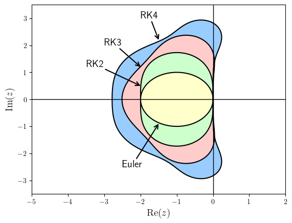
The regions of absolute stability for the Euler method and the explicit Runge-Kutta methods of order 2, 3 and 4 are plotted in Fig. 4.5.

Fig. 4.5 Regions of absolute stability for explicit Runge-Kutta methods of order 1 to 4.

Example 4.2

An explicit Runge-Kutta method is defined by the following Butcher tableau

\[\begin{split} \begin{align*}\begin{array}{c|cccc} 0 & & & & \\ 1/2 & 1/2 & & & \\ 3/4 & 0 & 3/4 & & \\ 1 & 2/9 & 1/3 & 4/9 & \\ \hline & 7/24 & 1/4 & 1/3 & 1/8 \end{array}\end{align*} \end{split}\]

(i) Determine the stability function for this Runge-Kutta method and hence find its order;

Solution (click to show)

Here we have

\[\begin{split} \begin{align*} A &= \begin{pmatrix} 0 & 0 & 0 & 0 \\ 1/2 & 0 & 0 & 0 \\ 0 & 3/4 & 0 & 0 \\ 2/9 & 1/3 & 4/9 & 0 \end{pmatrix}, & \vec{b} &= \begin{pmatrix} 7/24 \\ 1/4 \\ 1/3 \\ 1/8 \end{pmatrix}. \end{align*} \end{split}\]

Calculating \(\vec{b}^TA^{k - 1}\vec{e}\) for \(k = 1, \ldots, 4\)

\[\begin{split} \begin{align*} k &= 1, & \vec{b}^TA^0 \vec{e} &= \begin{pmatrix} 7/24 \\ 1/4 \\ 1/3 \\ 1/8 \end{pmatrix} \begin{pmatrix} 1 & 0 & 0 & 0 \\ 0 & 1 & 0 & 0 \\ 0 & 0 & 1 & 0 \\ 0 & 0 & 0 & 1 \end{pmatrix} \begin{pmatrix} 1 \\ 1 \\ 1 \\ 1 \end{pmatrix} = 1, \\ k &= 2, & \vec{b}^TA^1 \vec{e} &= \begin{pmatrix} 7/24 \\ 1/4 \\ 1/3 \\ 1/8 \end{pmatrix} \begin{pmatrix} 0 & 0 & 0 & 0 \\ 1/2 & 0 & 0 & 0 \\ 0 & 3/4 & 0 & 0 \\ 2/9 & 1/3 & 4/9 & 0 \end{pmatrix} \begin{pmatrix} 1 \\ 1 \\ 1 \\ 1 \end{pmatrix} = \frac{1}{2}, \\ k &= 3, & \vec{b}^TA^2 \vec{e} &= \begin{pmatrix} 7/24 \\ 1/4 \\ 1/3 \\ 1/8 \end{pmatrix} \begin{pmatrix} 0 & 0 & 0 & 0 \\ 0 & 0 & 0 & 0 \\ 3/8 & 0 & 0 & 0 \\ 1/6 & 1/3 & 0 & 0 \end{pmatrix} \begin{pmatrix} 1 \\ 1 \\ 1 \\ 1 \end{pmatrix} = \frac{3}{16}, \\ k &= 4, & \vec{b}^TA^3 \vec{e} &= \begin{pmatrix} 7/24 \\ 1/4 \\ 1/3 \\ 1/8 \end{pmatrix} \begin{pmatrix} 0 & 0 & 0 & 0 \\ 0 & 0 & 0 & 0 \\ 0 & 0 & 0 & 0 \\ 1/6 & 0 & 0 & 0 \end{pmatrix} \begin{pmatrix} 1 \\ 1 \\ 1 \\ 1 \end{pmatrix} = \frac{1}{48}. \end{align*} \end{split}\]

So the stability function is

\[ \begin{align*} R(z) = 1 + z + \frac{1}{2} z^2 + \frac{3}{16} z^3 + \frac{1}{48} z^4, \end{align*} \]

which agrees to the series expansion of \(e^z\) from equation (4.6) up to and including the \(z^2\) term. Therefore this method is of order 2.

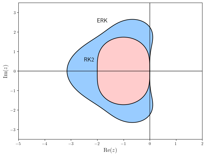
(ii) plot the region of absolute stability and that of an explicit method on the same order on the same set of axes;

Solution (click to show)

Code

Python

import numpy as np
import matplotlib.pyplot as plt
plt.rcParams['text.usetex'] = True

# Generate z values
xmin, xmax, ymin, ymax = -5, 2, -3.5, 3.5
X, Y = np.meshgrid(np.linspace(xmin, xmax, 200),np.linspace(ymin, ymax, 200))
Z = X + Y * 1j

# Define stability function
ERK = 1 + Z + 1/2 * Z ** 2 + 3/16 * Z ** 3 + 1/48 * Z ** 4
RK2 = 1 + Z + Z ** 2 / 2

# Plot stability region
fig = plt.figure(figsize=(8, 6))
plt.contourf(X, Y, abs(ERK), levels=[0, 1], colors="#99ccff")
plt.contour(X, Y, abs(ERK), colors= "k", levels=[0, 1])
plt.contourf(X, Y, abs(RK2), levels=[0, 1], colors="#ffcccc")
plt.contour(X, Y, abs(RK2), colors= "k", levels=[0, 1])
plt.axhline(0, color="k", linewidth=2)
plt.axvline(0, color="k", linewidth=2)
plt.axis([xmin, xmax, ymin, ymax])
plt.xlabel("$\mathrm{Re}(z)$", fontsize=14)
plt.ylabel("$\mathrm{Im}(z)$", fontsize=14)
plt.annotate("ERK", xy=(-1.5, 2.2), xytext=(-2, 3), fontsize=14, arrowprops=dict(arrowstyle="->", lw=1.5, shrinkA=0, shrinkB=0, ec="k"))
plt.annotate("RK2", xy=(-2, 0.5), xytext=(-3.5, 1.2), fontsize=14, arrowprops=dict(arrowstyle="->", lw=1.5, shrinkA=0, shrinkB=0, ec="k"))
plt.show()
:::

MATLAB

% Generate z values
xmin = -5;
xmax = 2;
ymin = -4;
ymax = 4;
[X, Y] = meshgrid(linspace(xmin, xmax, 200), linspace(ymin, ymax, 200));
Z = X + Y * 1i;

% Define stability function 
ERK = 1 + Z + 1/2 * Z .^ 2 + 3/16 * Z .^ 3 + 1/48 * Z .^ 4;
RK2 = 1 + Z + 1/2 * Z .^ 2;

% Plot the region of absolute stability
contour(X, Y, abs(ERK), [1, 1], 'b-', 'linewidth', 2)
hold on
contour(X, Y, abs(RK2), [1, 1], 'r-', 'linewidth', 2)
hold off
xline(0, LineWidth=2)
yline(0, LineWidth=2)
axis([xmin, xmax, ymin, ymax])
xlabel('$\mathrm{Re}(z)$', 'FontSize', 16, 'Interpreter', 'latex')
ylabel('$\mathrm{Im}(z)$', 'FontSize', 16, 'Interpreter', 'latex')
legend('ERK', 'RK2', FontSize=12)
:::

(iii) comment on the region of absolute stability of the two methods.

Solution (click to show)

The interval of absolute stability for this method is \([-3,0]\) whereas for the second-order method we have \([-2,0]\). This means that this method is stable for larger values of \(h\) so we can use fewer steps than the second-order method to calculate the solution to the same accuracy, although it does require the calculation of two additional stage values.