1.1. The Euler method

Fig. 1.2 Leonard Euler (1707 - 1783)

The Euler method, named after Swiss mathematician Leonhard Euler (pronounced “Oy-ler”), is the simplest numerical method used to solve ODEs. Consider the general first-order IVP

\[ y' = f(t, y), \qquad y(t_0) = y_0.\]

Since \(y'(t_0) = f(t_0, y_0)\), the solution curve has gradient \(f(t_0, y_0)\) at the point \((t_0, y_0)\). We approximate the solution locally by replacing the curve with its tangent line.

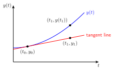
Fig. 1.3 The derivation of the Euler method.

The equation of the tangent line is

\[ y = y_0 + f(t_0, y_0) (t - t_0). \]

Let \(y_n\) denote a numerical approximation to the exact solution \(y(t_n)\). We can approximate the value of \(y_1\) by calculating the point on the tangent where \(t = t_1\)

\[ y_1 = y_0 + f(t_0, y_0) (t_1 - t_0). \]

We now treat the numerical approximation \(y_1\) as though it were the exact sotluion value at \(t_1\), allowing us to construct a new tangent approximation and continue the process. The gradient of the new tangent is \(f(t_1, y_1)\) so

\[ y_2 = y_1 + f(t_1, y_1) (t_2 - t_1). \]

Doing similar for more points along the \(t\) domain

\[\begin{split} \begin{align*} y_3 &= y_2 + f(t_2, y_2) (t_3 - t_2), \\ y_4 &= y_3 + f(t_3, y_3) (t_4 - t_3), \\ & \vdots \\ y_{n+1} &= y_n + f(t_n, y_n) (t_{n+1} - t_n). \end{align*} \end{split}\]

Let

\[ t_n = t_0 + nh, \qquad n = 0, 1, 2, \ldots \]

denote a sequence of equally spaced points in the domain where \(h\) is the step length and

\[ t_{n+1} = t_n + h.\]

The approximation of the solution to \(y_{n+1}\) is

\[ y_{n+1} = y_n + h f(t_n, y_n), \]

which is the Euler method.

Definition 1.3 (The Euler method)

The Euler method for solving the initial value problem \(y' = f(t, y)\), \(t \in [t_0, t_{\max}]\), \(y(t_0) = y_0\) is

(1.2)\[y_{n+1} = y_n + h f(t_n ,y_n),\]

where \(h = t_{n+1} - t_n\).

---

1.1.1. Solving an IVP using the Euler method

To solve an IVP using the Euler method we choose a value of the step length \(h\) and calculate the number of steps required to step through the domain \(t \in [t_0, t_{\max}]\). Using a constant step length \(h\) then \(t_n\) is

\[ t_n = t_0 + nh,\]

so

\[ n_{steps} = \frac{t_{\max} - t_0}{h} , \]

where \(n_{steps}\) is an integer. We then calculate \(y_1\) using equation (1.2) and \(t_1 = t_0 + h\). Then we use the values of \(t_1\) and \(y_1\) to calculate the values of \(y_2\) and \(t_2\) and continue this way until we have calculated \(y_n\) and \(t_n\) across the domain \([t_0, t_{\max}]\). The Euler method is an example of a single step method since it only requires information from a single step of the solution to calculate the next step. The other type of numerical method for solving ODEs is the linear multistep methods that requires information from multiple previous steps.

Algorithm 1.1 (Solving an IVP using the Euler method)

Inputs A first-order ODE of the form \(y' = f(t,y)\), a domain \(t \in [t_0, t_{\max}]\), an initial value \(y(t_0) = y_0\) and a step length \(h\)

Outputs \((t_0, t_1, \ldots)\) and \((y_0, y_1, \ldots)\)

• \(nsteps \gets \dfrac{t_{\max} - t_0}{h} \)

• For \(n = 0, \ldots, n_{steps} - 1\)

  • \(y_{n+1} \gets y_n + hf(t_n, y_n)\)

  • \(t_{n+1} \gets t_n + h\)

• Return \((t_0, t_1, \ldots)\) and \((y_0, y_1, \ldots)\)

Example 1.1

Calculate the solution to the following initial value problem using the Euler method with \(h = 0.2\)

\[y' = ty, \qquad t\in [0,1], \qquad y(0)=1.\]

---

Solution

Here the ODE function is \(f(t, y) = ty\), \(t_0 = 0\), \(y_0 = 1\) and \(h = 0.2\). First, we calculate the number of steps required

\[ nsteps = \left\lfloor \frac{t_{\max} - t_0}{h} \right\rfloor = \left\lfloor \frac{1 - 0}{0.2} \right\rfloor = 5. \]

We then step through the Euler method

\[\begin{split} \begin{align*} y_1 &= y_0 + h (t_0 y_0) = 1 + 0.2(0)(1) = 1, \\ t_1 &= t_0 + h = 0 + 0.2 = 0.2, \\ \\ y_2 &= y_1 + h (t_1 y_1) = 1 + 0.2(0.2)(1) = 1.04, \\ t_2 &= t_1 + h = 0.2 + 0.2 = 0.4, \\ \\ y_3 &= y_2 + h (t_2 y_2) = 1.04 + 0.2(0.4)(1.04) = 1.1232, \\ t_3 &= t_2 + h = 0.4 + 0.2 = 0.6, \\ \\ y_4 &= y_3 + h (t_3 y_3) = 1.1232 + 0.2(0.6)(1.1232) = 1.257984, \\ t_4 &= t_3 + h = 0.6 + 0.2 = 0.8, \\ \\ y_5 &= y_4 + h (t_4 y_4) = 1.257984 + 0.2(0.8)(1.257984) = 1.459261, \\ t_5 &= t_4 + h = 0.8 + 0.2 = 1.0. \end{align*} \end{split}\]

So the solution to this IVP using the Euler method is

\(t_n\)	\(y_n\)
0.00	1.000000
0.20	1.000000
0.40	1.040000
0.60	1.123200
0.80	1.257984
1.00	1.459261