3.3. Solving ODEs using Implicit Methods

Recall that the general form of an \(s\)-stage Runge-Kutta method is

(3.2)\[\begin{split} \begin{align*} y_{n+1} &= y_n + h \sum_{i = 1}^s b_i k_i, \\ k_i &= f(t_n + c_ih, y_n + h \sum_{j=1}^s a_{ij}k_j). \end{align*} \end{split}\]

Expanding out the summations in the stage values \(k_i\)

\[\begin{split} \begin{align*} k_1 &= f(t_n + c_1h, y_n + h (a_{11}k_1 + a_{12}k_2 + \cdots + a_{1s}k_s)), \\ k_2 &= f(t_n + c_2h, y_n + h (a_{21}k_1 + a_{22}k_2 + \cdots + a_{2s}k_s)), \\ & \vdots \\ k_s &= f(t_n + c_sh, y_n + h (a_{s1}k_1 + a_{s2}k_2 + \cdots + a_{ss}k_s)). \end{align*} \end{split}\]

The stage equations are implicit because the unknown stage values appear on both sides of the equations. So we need to recast the stage values so that we have a system of equations to solve. To make this easier we introduce a variable \(Y_i\) for the second parameter of \(f(t,y)\) in the stage value expressions, i.e.,

(3.3)\[ Y_i = y_n + h \sum_{j=1}^s a_{ij} k_j, \]

and the expression for the stage values \(k_i\) from (3.2) becomes

\[ k_i = f(t_n + c_ih, Y_i). \]

Substituting this into equation (3.3) gives

(3.4)\[ Y_i = y_n + h \sum_{j=1}^s a_{ij} f(t_n + c_jh, Y_j), \]

and also into equation (3.2) so the solution over a single step is

(3.5)\[ y_{n+1} = y_n + h \sum_{i=1}^s b_i f(t_n + c_ih, Y_i). \]

For a general non-linear function \(f(t, y)\), equation (3.4) is a system of \(s\) non-linear equations for the unknown stage values \(Y_1, \ldots Y_s\)​. In practice this system is usually solved using Newton’s method.

To demonstrate the solution using an IRK method we are going to consider the solution of the IVP

\[ y' = ty, \qquad t \in [0, 1], \qquad y(0) = 1, \]

using the third-order RadauIA method which has the Butcher tableau

\[\begin{split} \begin{array}{c|cc} 0 & \frac{1}{4} & -\frac{1}{4} \\ \frac{2}{3} & \frac{1}{4} & \frac{5}{12} \\ \hline & \frac{1}{4} & \frac{3}{4} \end{array} \end{split}\]

and a step length of \(h = 0.2\)

Substituting the coefficients for the Radau IA method into equation (3.4) we have

\[\begin{split} \begin{align*} Y_1 &= y_n + h ( \tfrac{1}{4} f(t_n, Y_1) - \tfrac{1}{4} f(t_n + \tfrac{2}{3}h, Y_2)), \\ Y_2 &= y_n + h ( \tfrac{1}{4} f(t_n, Y_1) + \tfrac{5}{12} f(t_n + \tfrac{2}{3}h, Y_2)). \end{align*} \end{split}\]

Since \(f(t, y) = ty\) then this becomes

\[\begin{split} \begin{align*} Y_1 &= y_n + h (\tfrac{1}{4} (t_nY_1) - \tfrac{1}{4} (t_n + \tfrac{2}{3}h)Y_2 ), \\ Y_2 &= y_n + h (\tfrac{1}{4} (t_nY_1) + \tfrac{5}{12} (t_n + \tfrac{2}{3}h)Y_2 ). \end{align*} \end{split}\]

This is a system of linear equations, so we can re-write this in the form \(A \mathbf{x} = \mathbf{b}\). Transposing the \(Y_i\) terms to on the left-hand side gives

\[\begin{split} \begin{align*} (1 - \tfrac{1}{4}ht_n)Y_1 + \tfrac{1}{4}h(t_n + \tfrac{2}{3}h)Y_2 &= y_n, \\ -\tfrac{1}{4}ht_nY_1 + (1 - \tfrac{5}{12}h(t_n + \tfrac{2}{3}h))Y_2 &= y_n. \end{align*} \end{split}\]

Writing this as a matrix equation

\[\begin{split} \begin{align*} \begin{pmatrix} 1 - \tfrac{1}{4}ht_n & \frac{1}{4}h(t_n + \frac{2}{3}h) \\ -\frac{1}{4}ht_n & 1 - \frac{5}{12}h(t_n + \frac{2}{3}h) \end{pmatrix} \begin{pmatrix} Y_1 \\ Y_2 \end{pmatrix} = \begin{pmatrix} y_n \\ y_n \end{pmatrix}. \end{align*} \end{split}\]

For the first step, \(t_0 = 0\), \(y_0 = 1\) and \(h = 0.2\) so

\[\begin{split} \begin{align*} \begin{pmatrix} 1 & 0.0067 \\ 0 & 0.9889 \end{pmatrix} \begin{pmatrix} Y_1 \\ Y_2 \end{pmatrix} = \begin{pmatrix} 1 \\ 1 \end{pmatrix}. \end{align*} \end{split}\]

Solving the linear system

\[\begin{split} \begin{align*} \begin{pmatrix} Y_1 \\ Y_2 \end{pmatrix} = \begin{pmatrix} 1 & 0.0067 \\ 0 & 0.9889 \end{pmatrix}^{-1} \begin{pmatrix} 1 \\ 1 \end{pmatrix} = \begin{pmatrix} 0.9933 \\ 1.0112 \end{pmatrix} \end{align*} \end{split}\]

So the stage values are \(Y_1 = 0.9933\) and \(Y_2 = 1.0112\). Note that although equation (3.4) is generally non-linear, for the test problem \(f(t,y)=ty\) the stage values appear only linearly, resulting in a linear system that can be solved directly.

The solution of the ODE \(y' = f(t, y)\) over a single time step using the third order RadauIA method is

\[y_{n+1} = y_n + h ( \tfrac{1}{4} f(t_n, Y_1) + \tfrac{3}{4} f(t_n + \tfrac{2}{3}h, Y_2)), \]

and since here \(y' = ty\) then

\[ y_{n+1} = y_n + h (\tfrac{1}{4} t_n Y_1 + \tfrac{3}{4} (t_n + \tfrac{2}{3}h) Y_2). \]

So the solution over the first step is

\[ \begin{align*} y_1 &= 1 + 0.2 (\tfrac{1}{4}(0)(0.9933) + \tfrac{3}{4}(0 + \tfrac{2}{3}(0.2))(1.0112)) = 1.0202. \end{align*} \]

The solution over the range \(t \in [0, 1]\) using the third-order Radau IA method is tabulated below and plotted against the exact solution in Fig. 3.1.

\(n\)	\(t_n\)	\(y_n\)	\(Y_1\)	\(Y_2\)
0	0.00	1.0000	-	-
1	0.20	1.0202	0.9933	1.0112
2	0.40	1.0833	1.0127	1.0598
3	0.60	1.1973	1.0740	1.1562
4	0.80	1.3773	1.1847	1.3131
5	1.00	1.6490	1.3592	1.5524

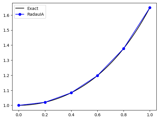
Fig. 3.1 The solution to the IVP \(y'=ty\), \(t \in [0,1]\), \(y(0)=1\) using the third-order Radau IA method with \(h=0.2\).