1.3. Error analysis

In Example 1.1 in the previous section we solved the following IVP using the Euler method

\[y' = ty, \qquad t\in [0,1], \qquad y(0)=1.\]

This IVP is quite simple we can use analytical methods to determine the solution which is \(y = e^{t^2/2}\). Since we have an exact solution we can calculate the absolute error between the numerical solution and the exact solution using

\[ \begin{align*} \text{absolute error} &= | y_\text{exact} - y_\text{numerical} |. \end{align*} \]

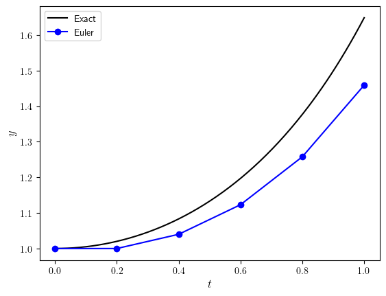
The numerical solution to this IVP computed using the Euler method, the exact solution for the same \(t\) values used in the Euler method and the absolute error are shown in Table 1.2 below and the numerical and exact solutions plotted in Fig. 1.5.

Table 1.2 Comparisons between the Euler method solutions and the exact solutions for the IVP \(y'=ty\), \(t\in[0,1]\), \(y(0)=1\).

\(t\)	Euler	Exact	Error
0.00	1.000000	1.000000	0.00e+00
0.2	1.000000	1.020201	2.02e-02
0.4	1.040000	1.083287	4.33e-02
0.6	1.123200	1.197217	7.40e-02
0.8	1.257984	1.377128	1.19e-0
1.0	1.459261	1.648721	1.89e-01

Fig. 1.5 Comparisons between the Euler method solutions and the exact solutions for the IVP \(y'=ty\), \(t\in[0,1]\), \(y(0)=1\).

From the Table 1.2 and Fig. 1.5 it is obvious that the numerical solution computed using the Euler method becomes increasingly inaccurate as \(t\) increases. This is because when deriving the Euler method we truncate the Taylor series so that any term after the first-order derivative is ignored. The omission of the higher-order terms means that the Taylor series is longer equal to \(f(t+h)\) and we have introduced an error. It is important that we study this error and the effect that the errors have on our solutions.

1.3.1. Changing the step length

Analysing the error of a numerical method is challenging since usually we do not know what the exact solution is (if we did we wouldn’t need a numerical method to calculate a solution). So instead we look at the behaviour of the error as the step length changes. Recall the Euler method which is

\[y_{n+1} = y_n + h f(t_n, y_n).\]

The solution over a single time step is changed from the current solution \(y_n\) by \(h\) multiplied by the value of \(f(t_n, y_n)\). If we assume that that value of \(y_n\) has some error associated to it then the error will also be changed by \(h\) multiplied by some value. Therefore, the smaller the value of \(h\) then the smaller the change in the error converging to zero when \(h\) is infinitesimally small.

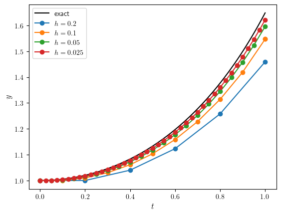
We can demonstrate this by looking at the solutions to the initial value problem from Example 1.1 using different values of the step length \(h\). The numerical solutions using \(h=0.2, 0.1, 0.05, 0.005\) have been plotted against the exact solution in Fig. 1.6.

Fig. 1.6 Solutions to the IVP \(y'=ty\), \(t \in [0,1]\), \(y(0)=1\) using the Euler method with step lengths \(h=0.2, 0.1, 0.05, 0.005\).

Here we can see that as the step length is reduced, the solution gets closer to the exact solution as expected. The absolute errors between the exact solution \(y(1) = e^{1/2} = 1.648721\ldots\) calculated using the different step lengths are tabulated in Table 1.3.

Table 1.3 Global truncation errors for Euler method uses different step lengths.

\(h\)	Euler	Error
0.2	1.459261	1.89e-01
0.1	1.547110	1.02e-01
0.05	1.595942	5.28e-02
0.025	1.621801	2.69e-02

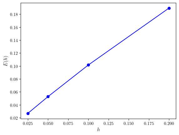
The third columns shows that as the step length is halved, the error decreases by a factor of approximately one half. This behaviour can be seen in Fig. 1.7 where the absolute errors between the numerical solutions for \(y(1)\) and the exact solution is plotted against the step length.

Fig. 1.7 Solutions to the IVP \(y'=ty\) using step lengths \(h=0.2, 0.1, 0.05, 0.005\).

1.3.2. Big-O notation

To compare the accuracy of different numerical methods we use big-O notation which describes the rate at which a function tends to zero.

Definition 1.5 (Big-O notation)

Let \(f(h) = O(h^n)\) then

\[\lim_{h \to 0} f(h) = Ch^n\]

for some positive constant \(C\).

If a function \(f(h)\) is \(f(h) = O(h^n)\) then we say that “f of h is big O of h to the power n” which means \(f(h)\) tends to zero at least as fast as \(h^n\). For example, if \(f(h) = O(h)\) then if we halve \(h\) then we would expect \(f(h)\) to also be halved (known as linear convergence), however if \(f(h) = O(h^2)\) then if we halve \(h\) then the value of \(f(h)\) would decrease by a factor of \(\frac{1}{4}\) since \((\frac{1}{2})^2 = \frac{1}{4}\) (known as quadratic convergence). So the higher the power of \(h\) the faster the function \(f(h)\) converges to zero as \(h\) decreases.

Since the error of a numerical method is dependent upon the step length \(h\) then we can say that it behaves like a polynomial function and we can approximate the error using \(f(h) = O(h^n)\).

Definition 1.6 (Order of a method)

If the error of a numerical method is \(O(h^n)\) then the method is said to be of order \(n\).

Note

The higher the order of a method, the more accurate the solution will be when using the same step length \(h\).

1.3.3. Local truncation error

Definition 1.7 (Local Truncation Error)

The Local Truncation Error (LTE), \(\tau_n\), is the error in the calculation of a single step of a numerical method assuming that the previous values used are exact.

Writing the Taylor series expansion for \(y(t)\) and if \(y'(t) = f(t, y)\) then

\[y(t + h) = y(t) + hf(t, y) + \frac{h^2}{2!}f'(t, y) + \cdots \]

When deriving the Euler method we truncated the Taylor series to first-order so

\[y_{n+1} = y_n + h f(t_n, y_n) + \tau_n,\]

where the local truncation error is

\[ \tau_n = \frac{h^2}{2!}f'(t_n, y_n) + \frac{h^3}{3!}f''(t_n, y_n) + \cdots \]

The value of the first term in \(\tau_n\) is much larger than that of all of the other terms so we can say that for the Euler method \(\tau_n = O(h^2)\).

1.3.4. Global truncation error

Definition 1.8 (Global Truncation Error)

The Global Truncation Error (GTE), \(E_n\), is the error that has accumulated over all previous steps of a numerical method assuming the initial solution was known to be exact.

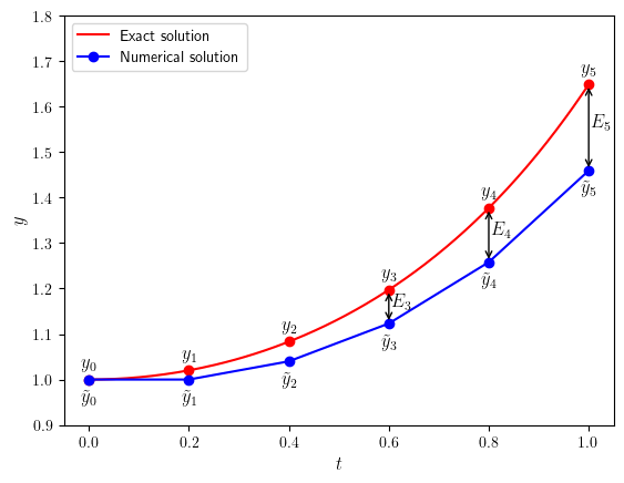
Let \(\tilde{y}_n\) denote a numerical solution and \(y_n\) denote the exact solution for \(y(t_n)\) then the global truncation error is calculated using

\[ \begin{align*} E_n = |y_n - \tilde{y}_n |, \end{align*} \]

This is represented graphically in Fig. 1.8.

Fig. 1.8 The global truncation error, \(E_n\), is the difference between the exact solution, \(y_n\), and the numerical solution, \(\tilde{y}_n\).

1.3.5. Accuracy of the Euler method

We can use the global and local truncations errors to analyse the accuracy of the Euler method. Comparing the exact, \(\tilde{y}\), and numerical solutions, \(y\), which are

\[\begin{split} \begin{align*} y_{n+1} &= y_{n} + hf(t_n, y_n), \\ \tilde{y}_{n+1} &= \tilde{y}_n + hf(t_n, \tilde{y}_n) + \tau_{n} \end{align*} \end{split}\]

and subtracting the first equation from the second gives

\[\begin{split} \begin{align*} y_{n+1} - \tilde{y}_{n+1} &= y_n - \tilde{y}_n + h(f(t_n, y_n) - f(t_n, \tilde{y}_n)) + \tau_{n} \\ E_{n+1} &= E_n + h(f(t_n, y_n) - f(t_n, \tilde{y}_n)) + \tau_{n} \end{align*} \end{split}\]

Assuming that \(f(t,y)\) satisfies the Lipschitz condition which is

\[ \begin{align*} |f(t_n, y_n) - f(t_{n+1}, y_{n+1})| \leq L|y_n - y_{n+1}|, \end{align*} \]

where \(L\) is the Lipschitz constant, then it can be shown that \(E_n\) satisfies

\[ \begin{align*} |E_n| \leq \frac{\displaystyle\max_i (\tau_i)}{h} \left(\frac{\exp(L(t_n - t_0)) - 1}{L}\right), \qquad i = 0, \ldots, n. \end{align*} \]

The term in the brackets is just some constant, \(C\) say, and since for the Euler method \(\tau = O(h^2)\) then

\[\begin{align*} E_n \leq C\frac{O(h^2)}{h} = O(h). \end{align*} \]

So this means the global truncation error for the Euler method is \(O(h)\) which confirms that it is a first order method. We saw in Fig. 1.7 that as \(h\) decreases the global truncation error decreased in a linear fashion where gradient of the line was approximately 1 confirming that the Euler method is a first-order method.

1.3.6. Code

The code used to produce Table 1.3 and Fig. 1.7 is shown below. This assumes the function solveIVP() and euler() have already been defined.

Python

# Define ODE function and the exact solution
def f(t,y):
    return t * y


def exact(t):
    return np.exp(t ** 2 / 2)


# Define IVP parameters
tspan = [0, 1]
y0 = [1]
hvals = [ 0.2, 0.1, 0.05, 0.025 ]  # step length values

# Loop through h values and calculate errors
errors = []
print(f"Exact solution: y(1) = {exact(1):0.6f}\n")
print("|   h   |  Euler   |  Error   |")
print("|:-----:|:--------:|:--------:|")
for h in hvals:
    t, y = solveIVP(f, tspan, y0, h, euler)
    errors.append(abs(y[-1,0] - exact(t[-1])))
    print(f"| {h:0.3f} | {y[-1,0]:0.6f} | {errors[-1]:0.2e} |")

# Plot errors
fig, ax = plt.subplots()
plt.plot(hvals, errors, "bo-")
plt.xlabel("$h$", fontsize=12)
plt.ylabel("$E(h)$", fontsize=12)
plt.show()

MATLAB

% Define ODE function and the exact solution
f = @(t, y) t * y;
exact = @(t) exp(t .^ 2 / 2);

% Define IVP parameters
tspan = [0, 1];
y0 = [1];
hvals = [0.2, 0.1, 0.05, 0.025];    % step length values

% Loop through h values and calculate solution
errors = [];
for i = 1 : 1 % use for loop to group print statements
    fprintf("Exact solution: y(1) = %1.6f", exact(1))
    fprintf(" ")
    fprintf("|   h   |  Euler   |  Error   |")
    fprintf("|:-----:|:--------:|:--------:|")
    for h = hvals
        [t, y] = solveIVP(f, tspan, y0, h, @euler);
        errors = [errors, abs(y(end) - exact(t(end)))];
        fprintf("| %1.3f | %1.6f | %1.2e |\n", h, y(end), errors(end))
    end
end
% Plot errors
plot(hvals, errors, 'b-o', LineWidth=2, MarkerFaceColor='b')
axis padded
xlabel('$h$', FontSize=14, Interpreter='latex')
ylabel('$E(h)$', FontSize=14, Interpreter='latex')