3.3. Solving Systems of ODEs using IRK Methods

On the previous page we saw that to solve a single ODE using an IRK method, we need to recast the stage value expressions as a linear system which is solved at each step of the method. When we have a system of multiple ODEs, this becomes more complicated as we need to do this for each equation in the system, and the stage values may form non-linear equations.

Consider the solution of the IVP of the form

\[\mathbf{y}' = \mathbf{f}(t, \mathbf{y}), \qquad t \in [t_0, t_{\max}], \qquad \mathbf{y}(0) = \mathbf{y}_0, \]

where

\[\begin{split} \begin{align*} \mathbf{y} &= \begin{pmatrix} y_1 \\ \vdots \\ y_N \end{pmatrix}, & \mathbf{f}(t, \mathbf{y}) &= \begin{pmatrix} f_1(t, \mathbf{y}) \\ \vdots \\ f_N(t, \mathbf{y}) \end{pmatrix}. \end{align*} \end{split}\]

Recall that the general form of a Runge-Kutta method for solving a system of ODEs is

(3.6)\[\begin{split} \begin{align*} \mathbf{y}_{n+1} &= \mathbf{y}_n + h \sum_{i=1}^s b_i \mathbf{k}_i,\\ \mathbf{k}_i &= \mathbf{f}(t_n +c_i h,\mathbf{y}_n + h \sum_{j=1}^s a_{ij} \mathbf{k}_j), \end{align*} \end{split}\]

In a similar approach to solving single ODEs, we introduce an \(N \times 1\) vector \(\mathbf{Y}_i\) for the solution of the system over intermediate intervals of the step

(3.7)\[\mathbf{Y}_i = \mathbf{y}_n + h \displaystyle\sum_{j=1}^s a_{ij} \mathbf{k}_j, \]

and the expression for the stage values \(\mathbf{k}_i\) becomes

\[\mathbf{k}_i = \mathbf{f}(t_n + c_ih, \mathbf{Y}_i). \]

Substituting this into equation (3.7) we have

(3.8)\[ \begin{align*} \mathbf{Y}_i = \mathbf{y}_n + h \sum_{j = 1}^s a_{ij} \mathbf{f}(t_n + c_j h, \mathbf{Y}_j). \end{align*} \]

and also into equation (3.6) gives

(3.9)\[ \begin{align*} \mathbf{y}_{n+1} &= \mathbf{y}_n + h \sum_{i=1}^s b_i \mathbf{f}(t_n + c_i h, \mathbf{Y}_i). \end{align*} \]

Using an \(s\)-stage IRK method, the values of \(\mathbf{Y}_i\) given by equation (3.8) are

(3.10)\[\begin{split} \begin{align*} \mathbf{Y}_1 &= \mathbf{y}_n + h (a_{11} \mathbf{f}(t_n + c_1h, \mathbf{Y}_1) + \cdots + a_{1s} \mathbf{f}(t_n + c_s h, \mathbf{Y}_s)), \\ \vdots \\ \mathbf{Y}_s &= \mathbf{y}_n + h (a_{s1} \mathbf{f}(t_n + c_1h, \mathbf{Y}_1) + \cdots + a_{ss} \mathbf{f}(t_n + c_s h, \mathbf{Y}_s)). \end{align*}\end{split}\]

Writing this as a matrix equation

(3.11)\[\begin{split} \begin{align*} \begin{pmatrix} \mathbf{Y}_1 \\ \vdots \\ \mathbf{Y}_s \end{pmatrix} = \begin{pmatrix} \mathbf{y}_n \\ \vdots \\ \mathbf{y}_n \end{pmatrix} + \begin{pmatrix} h a_{11} \mathbf{f}(t_n + c_1h, \mathbf{Y}_1) + \cdots + h a_{1s} \mathbf{f}(t_n + c_sh, \mathbf{Y}_s) \\ \vdots \\ h a_{s1} \mathbf{f}(t_n + c_1h, \mathbf{Y}_1) + \cdots + h a_{ss} \mathbf{f}(t_n + c_sh, \mathbf{Y}_s) \\ \end{pmatrix}. \end{align*} \end{split}\]

Since \(\mathbf{Y}_i\) are \(N \times 1\) vectors then these are \(sN \times 1\) vectors. We can replace the summation with matrix multiplications using a Kronecker product.

Definition 3.4 (The Kronecker product)

The Kronecker product between an \(m \times n\) matrix \(A\) and another \(p \times q\) matix \(B\) is denoted by \(A \otimes B\) and defined by

\[\begin{split} \begin{align*} A \otimes B = \begin{pmatrix} a_{11} B & \cdots & a_{1n} B \\ \vdots & \ddots & \vdots \\ a_{m1} B & \cdots & a_{mn} B \end{pmatrix}. \end{align*} \end{split}\]

In other words, each element of \(A\) is multiplied by the matrix \(B\).

For example, for a 2-stage method

\[\begin{split} \begin{align*} \begin{pmatrix} \mathbf{Y}_1 \\ \mathbf{Y}_2 \end{pmatrix} &= \begin{pmatrix} \mathbf{y}_n \\ \mathbf{y}_n \end{pmatrix} + h \begin{pmatrix} a_{11} \mathbf{f}(t_n + c_1h, \mathbf{Y}_1) + a_{12} \mathbf{f}(t_n + c_2h, \mathbf{Y}_2) \\ a_{21} \mathbf{f}(t_n + c_1h, \mathbf{Y}_1) + a_{22} \mathbf{f}(t_n + c_2h, \mathbf{Y}_2) \end{pmatrix}, \end{align*} \end{split}\]

Let’s say we have a system of \(N = 3\) ODEs. Introducing a notation where \(y_{j}\), \(Y_{i,j}\) and \(f_{i,j}\) are the \(j\)-th elements of \(\mathbf{y}_n\), \(\mathbf{Y}_i\) and \(\mathbf{f}(t_n + c_ih, \mathbf{Y}_i)\) respectively, then this can be written as

\[\begin{split} \begin{align*} \begin{pmatrix} Y_{1,1} \\ Y_{1,2} \\ Y_{1,3} \\ Y_{2,1} \\ Y_{2,2} \\ Y_{2,3} \end{pmatrix} &= \begin{pmatrix} y_{1} \\ y_{2} \\ y_{3} \\ y_{1} \\ y_{2} \\ y_{3} \end{pmatrix} + h \begin{pmatrix} a_{11} f_{1,1} + a_{12} f_{2,1} \\ a_{11} f_{1,2} + a_{12} f_{2,2} \\ a_{11} f_{1,3} + a_{12} f_{2,3} \\ a_{21} f_{1,1} + a_{22} f_{2,1} \\ a_{21} f_{1,2} + a_{22} f_{2,2} \\ a_{21} f_{1,3} + a_{22} f_{2,3} \end{pmatrix} \\ &= \begin{pmatrix} y_{1} \\ y_{2} \\ y_{3} \\ y_{1} \\ y_{2} \\ y_{3} \end{pmatrix} + h \begin{pmatrix} a_{11} & 0 & 0 & a_{12} & 0 & 0 \\ 0 & a_{11} & 0 & 0 & a_{12} & 0 \\ 0 & 0 & a_{11} & 0 & 0 & a_{12} \\ a_{21} & 0 & 0 & a_{22} & 0 & 0 \\ 0 & a_{21} & 0 & 0 & a_{22} & 0 \\ 0 & 0 & a_{21} & 0 & 0 & a_{22} \end{pmatrix} \begin{pmatrix} f_{1,1} \\ f_{1,2} \\ f_{1,3} \\ f_{2,1} \\ f_{2,2} \\ f_{2,3} \end{pmatrix} \end{align*} \end{split}\]

The \(6 \times 6\) matrix is \(A \otimes I_N\) so we can write the expression for the stage values \(\mathbf{Y}_i\) as

(3.12)\[ \mathbf{Y} = \mathbf{e} \otimes \mathbf{y}_n + h (A \otimes I_N) F(\mathbf{Y}), \]

where

\[\begin{split} \begin{align*} \mathbf{Y} &= \begin{pmatrix} \mathbf{Y}_1 \\ \vdots \\ \mathbf{Y}_s \end{pmatrix}, & \mathbf{e} &= \begin{pmatrix} 1 \\ \vdots \\ 1 \end{pmatrix}, & F(\mathbf{Y}) &= \begin{pmatrix} \mathbf{f}(t_n + c_1h, \mathbf{Y}_1) \\ \vdots \\ \mathbf{f}(t_n + c_s h, \mathbf{Y}_s) \end{pmatrix}. \end{align*} \end{split}\]

We can also use a Kronecker product to simplify the expression for the summation in (3.9)

(3.13)\[ \mathbf{y}_{n+1} = \mathbf{y}_n + h (\mathbf{b}^\mathsf{T} \otimes I_N) F(\mathbf{Y}). \]

---

3.3.1. Newton’s method

To compute the stage values \(\mathbf{Y}_1, \ldots, \mathbf{Y}_s\)​, we must solve the system given in equation (3.12). Unlike the examples in the previous page, this system is generally nonlinear because the function \(\mathbf{f}(t,\mathbf{y})\) may contain nonlinear terms. This means we cannot rearrange the equations into a linear system and solve them directly. To solve these equations we use Newton’s method, which is a well known numerical method to computing the solutions of \(g(x) = 0\) where \(g\) is a differentiable function.

3.3.1.1. Newton’s method for a single equation

Suppose we wish to solve

\[ g(x) = 0. \]

Starting from an initial guess value \(x^{(0)}\), Newton’s method repeatedly improves the estimate using

\[x^{(k+1)} = x^{(k)} - \frac{g(x^{(k)})}{g'(x^{(k)})}. \]

The iterations continue until successive estimates differ by less than a specified tolerance.

3.3.1.2. Newton’s method for a system of equations

Given a system of equations \(g(\mathbf{x}) = \mathbf{0}\) where \(g = (g_1, g_2, \ldots)\) are differentiable functions, then the matrix form of Newton’s method is

\[\mathbf{x}^{(k+1)} = \mathbf{x}^{(k)} - J^{-1}g(\mathbf{x}^{(k)}),\]

where \(J\) is the Jacobian matrix

\[\begin{split} \begin{align*} J = \frac{\partial g}{\partial \mathbf{x}} = \begin{pmatrix} \dfrac{\partial g_1}{\partial x_1} & \cdots & \dfrac{\partial g_1}{\partial x_N} \\ \vdots & \ddots & \vdots \\ \dfrac{\partial g_N}{\partial x_1} & \cdots & \dfrac{\partial g_N}{\partial x_N} \end{pmatrix}. \end{align*} \end{split}\]

Rather than computing the inverse \(J^{-1}\), which is expensive and unnecessary, we solve the linear system

\[J \Delta x = -g(\mathbf{x}^{(k)}), \]

where

\[ \Delta \mathbf{x} = \mathbf{x}^{(k + 1)} - \mathbf{x}^{(k)}. \]

Once \(\Delta \mathbf{x}\) has been found, the estimate is improved using

The improved estimate is then calculated using

\[ \mathbf{x}^{(k+1)} = \mathbf{x}^{(k)} + \Delta \mathbf{x}. \]

This process is repeated until

\[ \| \Delta \mathbf{x} \| < tol.\]

3.3.1.3. Computing the stage values using Newton’s method

For an \(s\)-stage IRK method applied to a system of \(N\) ODEs, the unknown vector

\[\begin{split} \mathbf{Y} = \begin{pmatrix} \mathbf{Y}_1 \\ \vdots \\ \mathbf{Y}_2 \end{pmatrix}, \end{split}\]

contains \(sN\) unknowns. We rewrite the stage equations (3.12) as

(3.14)\[ G(\mathbf{Y}) = \mathbf{Y} - \mathbf{e} \otimes \mathbf{y}_n - h(A \otimes I_N) F(\mathbf{Y}),\]

The Jacobian matrix is

\[ \begin{align*} J_G &= \frac{\partial G}{\partial \mathbf{Y}} = I_{sN} - h(A \otimes I_N) F'(\mathbf{Y}), \end{align*} \]

where

\[\begin{split} F'(\mathbf{Y}) = \begin{pmatrix} J_f^{(1)} & 0 & \cdots & 0 \\ 0 & J_f^{(2)} & \ddots & \vdots \\ \vdots & \ddots & \ddots & 0 \\ 0 & \cdots & 0 & J_f^{(s)} \end{pmatrix}, \end{split}\]

and

\[ J_f^{(i)} = \frac{\partial}{\partial \mathbf{y}} \mathbf{f}(t_n + c_ih, \mathbf{Y}_i).\]

Each Jacobian \(J_f^{(i)}\) is an \(N \times N\) matrix so \(J_G\) is an \(sN \times sN\) matrix

\[\begin{split} \begin{align*} J_G &= I_{sN} - h \begin{pmatrix} a_{11} J_f^{(1)} & \cdots & a_{1s} J_f^{(s)} \\ \vdots & \ddots & \vdots \\ a_{s1} J_f^{(1)} & \cdots & a_{ss} J_f^{(s)} \end{pmatrix}. \end{align*} \end{split}\]

Computing \(J_f^{(1)}, \ldots, J_f^{(s)}\) at every Newton iteration can be expensive. A common simplification is

\[ J_f^{(i)} \approx \frac{\partial}{\partial \mathbf{y}} \mathbf{f}(t_n, \mathbf{y}_n)\]

so equation (3.14) becomes

\[ J_G = I_{sN} - h (A \otimes J_f). \]

3.3.1.4. Computing \(J_f\)

The individual \(J_f\) Jacobians can be computed using a finite difference approximation

\[ J_{f}^{(i)} = \frac{\partial}{\partial y_i} \mathbf{f}(t_n, \mathbf{y}_n)\approx \frac{\mathbf{f}(t_n, \mathbf{y}_n + \epsilon \, \mathbf{e}_i) - \mathbf{f}(t_n, \mathbf{y}_n)}{\epsilon \,},\]

where \(\mathbf{\epsilon}\) is some small value and \(\mathbf{e}_i\) is column \(i\) of \(I_s\). For example, consider a system of two ODEs

\[\begin{split} \begin{align*} \mathbf{f}(t, \mathbf{y}) = \begin{pmatrix} f_1(t, y_1, y_2) \\ f_2(t, y_1, y_2) \end{pmatrix}. \end{align*} \end{split}\]

The Jacobian is

\[\begin{split} J_f = \begin{pmatrix} \dfrac{\partial f_1}{\partial y_1} & \dfrac{\partial f_1}{\partial y_2} \\ \dfrac{\partial f_2}{\partial y_1} & \dfrac{\partial f_2}{\partial y_2} \end{pmatrix}. \end{split}\]

To approximate the first column, we only perturb \(y_1\)

\[ \frac{\partial}{\partial y_1} \mathbf{f}(t, \mathbf{y}) \approx \frac{\mathbf{f}(t, \mathbf{y} + \epsilon \, \mathbf{e}_1) - \mathbf{f}(t, \mathbf{y})}{\epsilon \,}, \]

where

\[\begin{split} \mathbf{y} + \epsilon \, \mathbf{e}_1 = \begin{pmatrix} y_1 \\ y_2 \end{pmatrix} + \epsilon \, \begin{pmatrix} 1 \\ 0 \end{pmatrix} = \begin{pmatrix} y_1 + \epsilon \, \\ y_2 \end{pmatrix}. \end{split}\]

To approximate the second column, we only perturb \(y_2\)

\[ \frac{\partial}{\partial y_2}\mathbf{f}(t, \mathbf{y}) \approx \frac{\mathbf{f}(t, \mathbf{y} + \epsilon \, \mathbf{e}_2) - \mathbf{f}(t, \mathbf{y})}{\epsilon \,}, \]

where

\[\begin{split} \mathbf{y} + \epsilon \, \mathbf{e}_2 = \begin{pmatrix} y_1 \\ y_2 \end{pmatrix} + \epsilon \, \begin{pmatrix} 0 \\ 1 \end{pmatrix} = \begin{pmatrix} y_1 \\ y_2 + \epsilon \, \end{pmatrix}. \end{split}\]

The Jacobian matrix \(J_f\) is constant for all Newton iterations, so the solution of the linear system is well suited to LU decomposition.

---

3.3.2. Applying an IRK to solve a system of ODEs

The steps used to solve an IVP using an IRK method are outlined in Algorithm 3.1.

Algorithm 3.1 (Solving an IVP using an IRK method)

Inputs A system of \(N\) first-order ODEs of the form \(\mathbf{y}' = \mathbf{f}(t, \mathbf{y})\), a domain \(t \in [t_0, t_{\max}]\), a vector of initial values \(\mathbf{y}(t_0) = y_0\) and a value of the step length \(h\)

Outputs \((t_0, t_1, \ldots)\) and \((\mathbf{y}_0, \mathbf{y}_1, \ldots)\).

• \(\mathbf{e} = (1, \ldots, 1)^\mathsf{T} \in \mathbb{R}^s\)

• \(n_{steps} \gets \dfrac{t_{\max} - t_0}{h}\)

• For \(n = 0, \ldots, n_{steps}\)

  • \(\mathbf{Y} \gets \mathbf{e} \otimes \mathbf{y}_n\)

  • \(J_f \gets \dfrac{\partial}{\partial \mathbf{y}} \mathbf{f}(t_n, \mathbf{y}_n)\)

  • \(J_G \gets I_{sN} - h (A \otimes J_f)\)

  • For \(k = 1, \ldots, maxiter\)

    • \(F(\mathbf{Y}) \gets \begin{pmatrix} \mathbf{f}(t_n + c_1h, \mathbf{Y}_1) \\ \vdots \\ \mathbf{f}(t_n + c_sh, \mathbf{Y}_s) \end{pmatrix}\)

    • \(G(\mathbf{Y}) \gets \mathbf{Y} - \mathbf{e} \otimes \mathbf{y}_n - h (A \otimes I_N) F(\mathbf{Y})\)

    • Solve the linear system \(J_G \Delta \mathbf{Y} = -G(\mathbf{Y})\) for \(\Delta \mathbf{Y}\)

    • \(\mathbf{Y} \gets \mathbf{Y} + \Delta \mathbf{Y}\)

    • If \(\| \Delta \mathbf{Y} \| < tol\)

      • break

  • \(\mathbf{y}_{n+1} \gets \mathbf{y}_n + h (\mathbf{b}^T \otimes I_N) F(\mathbf{Y})\)

  • \(t_{n+1} \gets t_n + h\)

• Return \((t_0, t_1, \ldots)\) and \((\mathbf{y}_0, \mathbf{y}_1, \ldots)\)

The additional cost of solving an \(sN\)-dimensional nonlinear system at every step is compensated by the excellent stability properties of IRK methods, making them particularly effective for stiff systems of ODEs.

Example 3.4

The van der Pol oscillator is a well known model of an oscillating system with non-linear damping described by the second-order ODE

\[ \ddot{y} - \mu (1 - y^2) \dot{y} + y = 0, \]

where \(\mu\) is a scalar parameter that governs the strength of the damping.

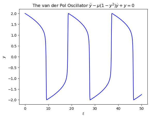
Use the Radau IA method to compute the solution to the van der Pol oscillator over the first 50 seconds where \(y(0) = 2\) and \(\mu = 10\) using a step length of \(h = 0.1\) and a convergence tolerance of \(tol = 10^{-4}\) for Newton’s method.

---

Solution

We need to rewrite the second-order ODE as a system of first-order ODEs. Let \(y_1 = y\) and \(y_2 = \dot{y}_1\) then

\[\begin{split} \begin{align*} \dot{y}_1 &= y_2, \\ \dot{y}_2 &= \mu (1 - y_1^2) y_2 - y_1, \end{align*} \end{split}\]

so

\[\begin{split} \begin{align*} \mathbf{y}&= \begin{pmatrix} y_1 \\ y_2 \end{pmatrix}, & \mathbf{f}(t, \mathbf{y}) &= \begin{pmatrix} y_2 \\ \mu (1 - y_1^2) y_2 - y_1 \end{pmatrix}. \end{align*} \end{split}\]

The coefficients for the Radau IA method are

\[\begin{split} \begin{align*} A &= \begin{pmatrix} \frac{1}{4} & -\frac{1}{4} \\ \frac{1}{4} & \frac{5}{12} \end{pmatrix}, & \mathbf{b} &= \begin{pmatrix} \frac{1}{4} \\ \frac{3}{4} \end{pmatrix} & \mathbf{c} &= \begin{pmatrix} 0 \\ \frac{2}{3} \end{pmatrix}. \end{align*} \end{split}\]

The initial conditions are \(\mathbf{y}_0 = (2, 0)\) and \(\mu = 10\). The Jacobian matrix of the ODE system for the first step is

\[\begin{split} \begin{align*} J_f &= \begin{pmatrix} 0 & 1 \\ -2\mu y_1y_2 - 1 & \mu(1 - y_1^2) \end{pmatrix} = \begin{pmatrix} 0 & 1 \\ -2(10)(2)(0) - 1 & 10(1 - 2^2) \end{pmatrix} = \begin{pmatrix} 0 & 1 \\ -1 & -30 \end{pmatrix}, \end{align*} \end{split}\]

so the Jacobian used in the Newton iterations for the first step is

\[\begin{split} \begin{align*} J_G &= I_4 - h (A \otimes J_f) = \begin{pmatrix} 1 & 0 & 0 & 0 \\ 0 & 1 & 0 & 0 \\ 0 & 0 & 1 & 0 \\ 0 & 0 & 0 & 1 \end{pmatrix} - 0.1 \begin{pmatrix} 0 & \frac14 & 0 & -\frac14 \\ -\frac14 & -\frac{15}{2} & \frac14 & \frac{15}{2} \\ 0 & \frac14 & 0 & \frac{5}{12} \\ -\frac14 & -\frac{15}{2} & -\frac{5}{12} & -\frac{25}{2} \end{pmatrix} \\ &= \begin{pmatrix} 1 & -\frac{1}{40} & 0 & \frac{1}{40} \\ \frac{1}{40} & \frac74 & -\frac{1}{40} & -\frac34 \\ 0 & -\frac{1}{40} & 1 & -\frac{1}{24} \\ \frac{1}{40} & \frac34 & \frac{1}{24} & \frac94 \end{pmatrix}, \end{align*} \end{split}\]

Computing \(\mathbf{Y}\), \(F(\mathbf{Y})\) and \(G(\mathbf{Y})\)

\[\begin{split} \begin{align*} \mathbf{Y} &= \mathbf{e} \otimes \mathbf{y}_0 = \begin{pmatrix} 1 \\ 1 \end{pmatrix} \otimes \begin{pmatrix} 2 \\ 0 \end{pmatrix}= \begin{pmatrix} 2 \\ 0 \\ 2 \\ 0 \end{pmatrix}, \\ F(\mathbf{Y}) &= \begin{pmatrix} \mathbf{f}(t_0 + 0h, \mathbf{Y}_1) \\ \mathbf{f}(t_0 + \frac{2}{3}h, \mathbf{Y}_2) \end{pmatrix} = \begin{pmatrix} 0 \\ 10(1 - 2^2)(0) - 2 \\ 0 \\ 10(1 - 2^2)(0) - 2 \end{pmatrix} = \begin{pmatrix} 0 \\ -2 \\ 0 \\ -2 \end{pmatrix} \\ G(\mathbf{Y}) &= \mathbf{Y} - \mathbf{e} \otimes \mathbf{y}_n - h(A \otimes I_2) F(\mathbf{Y}) \\ &= \begin{pmatrix} 2 \\ 0 \\ 2 \\ 0 \end{pmatrix} - \begin{pmatrix} 2 \\ 0 \\ 2 \\ 0 \end{pmatrix} - 0.1 \begin{pmatrix} \frac{1}{4} & 0 & -\frac{1}{4} & 0 \\ 0 & \frac{1}{4} & 0 & -\frac{1}{4} \\ \frac{1}{4} & 0 & \frac{5}{12} & 0 \\ 0 & \frac{1}{4} & 0 & \frac{5}{12} \end{pmatrix} \begin{pmatrix} 0 \\ -2 \\ 0 \\ -2 \end{pmatrix} = \begin{pmatrix} 0 \\ 0 \\ 0 \\ \frac{2}{15} \end{pmatrix}. \\ \end{align*} \end{split}\]

Solving the linear system \(J_G \Delta \mathbf{Y} = -G(\mathbf{Y})\) gives

\[\begin{split} \begin{align*} \Delta \mathbf{Y} &= \begin{pmatrix} 1 & -\frac{1}{40} & 0 & \frac{1}{40} \\ \frac{1}{40} & \frac74 & -\frac{1}{40} & -\frac34 \\ 0 & -\frac{1}{40} & 1 & -\frac{1}{24} \\ \frac{1}{40} & \frac34 & \frac{1}{24} & \frac94 \end{pmatrix}^{-1} \begin{pmatrix} 0 \\ 0 \\ 0 \\ -\frac{2}{15} \end{pmatrix} = \begin{pmatrix} 0.0007 \\ -0.0222 \\ -0.0027 \\ -0.0518 \end{pmatrix}. \end{align*} \end{split}\]

The new estimate of \(\mathbf{Y}\) is

\[\begin{split} \begin{align*} \mathbf{Y} &= \mathbf{Y} + \Delta \mathbf{Y} = \begin{pmatrix} 2 \\ 0 \\ 2 \\ 0 \end{pmatrix} + \begin{pmatrix} 0.0007 \\ -0.0222 \\ -0.0027 \\ -0.0518 \end{pmatrix} = \begin{pmatrix} 2.0007 \\ -0.0222 \\ 1.9973 \\ -0.0518 \end{pmatrix} \end{align*}. \end{split}\]

Here \(\|\Delta \mathbf{Y}\| = 0.056447 > 10^{-4}\) so we need to continue iterating. Computing \(F(\mathbf{Y})\) and \(G(\mathbf{Y})\) using the new values of \(\mathbf{Y}\)

\[\begin{split} \begin{align*} F(\mathbf{Y}) &= \begin{pmatrix} \mathbf{f}(t_0 + 0h, \mathbf{Y}_1) \\ \mathbf{f}(t_0 + \frac{2}{3}h, \mathbf{Y}_2) \end{pmatrix} = \begin{pmatrix} -0.0222 \\ 10(1 - 2.0007^2)(-0.0222) - 2.0007 \\ -0.0518 \\ 10(1 - 1.9973^2)(-0.0518) - 1.9973 \end{pmatrix} = \begin{pmatrix} -0.0222 \\ -1.3326 \\ -0.0518 \\ -0.4489 \end{pmatrix} \\ G(\mathbf{Y}) &= \mathbf{Y} - \mathbf{e} \otimes \mathbf{y}_n - h(A \otimes I_2) F(\mathbf{Y}) \\ &= \begin{pmatrix} 2.0007 \\ -0.0222 \\ 1.9973 \\ -0.0518 \end{pmatrix} - \begin{pmatrix} 2 \\ 0 \\ 2 \\ 0 \end{pmatrix} - 0.1 \begin{pmatrix} \frac{1}{4} & 0 & -\frac{1}{4} & 0 \\ 0 & \frac{1}{4} & 0 & -\frac{1}{4} \\ \frac{1}{4} & 0 & \frac{5}{12} & 0 \\ 0 & \frac{1}{4} & 0 & \frac{5}{12} \end{pmatrix} \begin{pmatrix} -0.0222 \\ -1.3326 \\ -0.0518 \\ -0.4489 \end{pmatrix} = \begin{pmatrix} 0 \\ -0.0002 \\ 0 \\ -0.0002 \end{pmatrix}. \\ \end{align*} \end{split}\]

Solving the linear system \(J_G \Delta \mathbf{Y} = -G(\mathbf{Y})\) gives

\[\begin{split} \begin{align*} \Delta \mathbf{Y} &= \begin{pmatrix} 1 & -\frac{1}{40} & 0 & \frac{1}{40} \\ \frac{1}{40} & \frac74 & -\frac{1}{40} & -\frac34 \\ 0 & -\frac{1}{40} & 1 & -\frac{1}{24} \\ \frac{1}{40} & \frac34 & \frac{1}{24} & \frac94 \end{pmatrix}^{-1} \begin{pmatrix} 0 \\ 0.0002 \\ 0 \\ 0.0002 \end{pmatrix} = \begin{pmatrix} 0 \\ 0 \\ 0 \\ -0.0001 \end{pmatrix}, \end{align*} \end{split}\]

The new estimate of \(\mathbf{Y}\) is

\[\begin{split} \begin{align*} \mathbf{Y} &= \mathbf{Y} + \Delta \mathbf{Y} = \begin{pmatrix} 2.0007 \\ -0.0222 \\ 1.9973 \\ -0.0518 \end{pmatrix} + \begin{pmatrix} 0 \\ 0 \\ 0 \\ -0.0001 \end{pmatrix} = \begin{pmatrix} 2.0007 \\ -0.0222 \\ 1.9973 \\ -0.0519 \end{pmatrix} \end{align*}. \end{split}\]

Now \(\| \Delta(\mathbf{Y}) \| = 1.1864 \times 10^{-4} > 10^{-4}\) so we need to keep iterating. One more iteration results in \(\Delta \mathbf{Y} = \mathbf{0}\) (correct to 4 significant figures) so

\[\begin{split} \begin{align*} \mathbf{Y} &= \begin{pmatrix} 2.0007 \\ -0.0222 \\ 1.9973 \\ -0.0519 \end{pmatrix}, & F(\mathbf{Y}) &= \begin{pmatrix} -0.0222 \\ -1.3339 \\ -0.0519 \\ -0.4456 \end{pmatrix}. \end{align*} \end{split}\]

We can now compute the solution over the first step

\[\begin{split} \begin{align*} \mathbf{y}_1 &= \mathbf{y_0} + h(\mathbf{b}^\mathsf{T} \otimes I_2) F(\mathbf{Y}) \\ &= \begin{pmatrix} 2 \\ 0 \end{pmatrix} + 0.1 \begin{pmatrix} \frac{1}{4} & 0 & \frac{3}{4} & 0 \\ 0 & \frac{1}{4} & 0 & \frac{3}{4} \end{pmatrix} \begin{pmatrix} -0.0222 \\ -1.3339 \\ -0.0519 \\ -0.4456 \end{pmatrix} = \begin{pmatrix} 1.9956 \\ -0.0667 \end{pmatrix}. \end{align*} \end{split}\]

The solution over the full domain \(t \in [0, 50]\) is shown in Fig. 3.2.

Fig. 3.2 Solution of the van der Pol oscillator where \(\mu=10\) using the Radau IA IRK method.

---

3.3.3. Code

The code below defines the functions jac() and radauIA() which computes the Jacobian of a function \(\mathbf{f}(t, y)\) and the solution to an initial value problem using the Radau IA method respectively.

Python

def jac(f, t, y):
    N = len(y)
    J = np.zeros((N, N))
    I = np.eye(N)
    epsilon = 1e-6
    
    for i in range(N):
        J[:,i] = (f(t, y + epsilon * I[:,i]) - f(t,y)) / epsilon

    return J


def radauIA(f, tspan, y0, h):
    
    # Determine the number of ODEs in the system
    N = len(y0)

    # Calculate the number of steps required
    nsteps = int((tspan[1] - tspan[0]) / h)

    # Define solution arrays and assign initial values
    t = np.zeros(nsteps + 1)
    y = np.zeros((nsteps + 1, N))
    t[0] = tspan[0]
    y[0,:] = y0
    
    # Define Butcher tableau
    A = np.array([[1/4, -1/4],
                  [1/4, 5/12]])
    b = np.array([1/4, 3/4])
    c = np.array([0, 2/3])
    s = 2

    e = np.ones(s)
    
    # Define maximum Newton iterations
    max_iter = 10

    # Loop through steps
    for n in range(nsteps):

        # Use Newton's method to solve for the stage values
        Y = np.kron(e, y[n,:])
        F = np.zeros(s * N)
        Jf = jac(f, t[n], y[n,:])
        JG = np.eye(s * N) - h * np.kron(A, Jf)

        for k in range(max_iter):
            for i in range(s):
                idx = slice(i * N, (i + 1) * N)
                F[idx] = f(t[n] + c[i] * h, Y[idx])

            G = Y - np.kron(e, y[n,:]) - h * np.kron(A, np.eye(N)) @ F
            delta_Y = np.linalg.solve(JG, -G)
            Y += delta_Y

            if np.linalg.norm(delta_Y) < 1e-6:
                break

        y[n+1,:] = y[n,:] + h * np.kron(b.T, np.eye(N)) @ F
        t[n+1] = t[n] + h

    return t, y

This code uses the following NumPy functions:

• np.eye(N) – returns \(I_N\)

• np.kron(A, B) – returns the Kronecker product \(A \otimes B\)

• np.linalg.solve(A, b) – returns the solution to the linear system \(A \mathbf{x} = \mathbf{b}\)

• np.eye(n) – returns the \(n \times n\) identity matrix

• np.linalg.norm(a) – returns the Euclidean norm of the vector \(\mathbf{a}\)

MATLAB

function J = jac(f, t, y)

N = length(y);
J = zeros(N, N);
I = eye(N);
epsilon = 1e-6;

for i = 1 : N
    J(:, i) = (f(t, y + epsilon * I(:,i)) - f(t, y)) / epsilon;
end

end

function [t, y] = radauIA(f, tspan, y0, h)

% Determine the number of ODEs in the system
N = length(y0);

% Calculate the number of steps required
nsteps = floor((tspan(2) - tspan(1)) / h);

% Define solution arrays and assign initial values
t = zeros(nsteps + 1, 1);
y = zeros(nsteps + 1, N);
t(1) = tspan(1);
y(1,:) = y0;

% Define Butcher tableau
A = [ 1/4, -1/4 ; 1/4, 5/12 ];
b = [ 1/4 ; 3/4 ];
c = [ 0 ; 2/3 ];
s = 2;
e = ones(s, 1);

% Define maximum Newton iterations
max_iter = 10;

% Loop through steps
for n = 1 : nsteps

    % Use Newton's method to solve for the stage values
    Y = kron(e, y(n,:)');
    F = zeros(s * N, 1);
    Jf = jac(f, t(n), y(n,:)');
    JG = eye(s * N) - h * kron(A, Jf);

    for k = 1 : max_iter
        for i = 1 : s
            idx = 1 + (i - 1) * N : i * N;
            F(idx) = f(t(n) + c(i) * h, Y(idx)');
        end
        G = Y - kron(e, y(n,:)') - h * kron(A, eye(N)) * F;
        delta_Y = JG \ -G;
        Y = Y + delta_Y;

        if norm(delta_Y) < 1e-6
            break
        end
    end

    y(n+1,:) = y(n,:) + (h * kron(b', eye(N)) * F)';
    t(n+1) = t(n) + h;
end

end

This code uses the following functions:

• eye(N) – returns \(I_N\)

• kron(A, B) – returns the Kronecker product \(A \otimes B\)

• A \ b – returns the solution to the linear system \(A \mathbf{x} = \mathbf{b}\)

• eye(n) – returns the \(n \times n\) identity matrix

• norm(a) – returns the Euclidean norm of the vector \(\mathbf{a}\)

Note

The solution of the linear system for Newton’s method in the code above was done using NumPy’s and MATLAB’s linear system solvers. In practice, this is done using LU decomposition which is more efficient in this case since the coefficient method is constant for all iterations in a step. I used NumPy’s and MATLAB’s solvers here since have yet to meet LU decomposition which is covered in a later chapters.