6.5. Surface plots#
To create a 3D plot we first need to create a 3D axis using the Axes3D toolkit which is done using the following commands.
from mpl_toolkits.mplot3d import Axes3D

fig = plt.figure()
ax = plt.axes(projection='3d')
Surface plots can then be generated using the ax.plot_surface() function
ax.plot_surface(X, Y, Z)
where X, Y and Z are 2D co-ordinate arrays. To produce a surface plot of the bi-variate function \(z=f(x,y)\) we require \(x\) and \(y\) co-ordinates in the domain. The np.meshgrid() function is useful for generating these.
X, Y = np.meshgrid(x, y)
This generates two 2D arrays X and Y from two 1D arrays x and y. X contains the elements of x arranged in rows and Y contains the elements of y arranged in columns. To demonstrate this enter the following code into your program.
# Mesh grid
x = np.linspace(0, 4, 5)
y = np.linspace(0, 3, 4)
X, Y = np.meshgrid(x, y)

print()
print(f"x = {x}")
print(f"y = {y}")
print(f"\nX = \n{X}")
print(f"\nY = \n{Y}")
Run your program and you should see the following added to the console.
6.5 Mesh grid
-------------
x = [0. 1. 2. 3. 4.]
y = [0. 1. 2. 3.]

X =
[[0. 1. 2. 3. 4.]
 [0. 1. 2. 3. 4.]
 [0. 1. 2. 3. 4.]
 [0. 1. 2. 3. 4.]]

Y =
[[0. 0. 0. 0. 0.]
 [1. 1. 1. 1. 1.]
 [2. 2. 2. 2. 2.]
 [3. 3. 3. 3. 3.]]
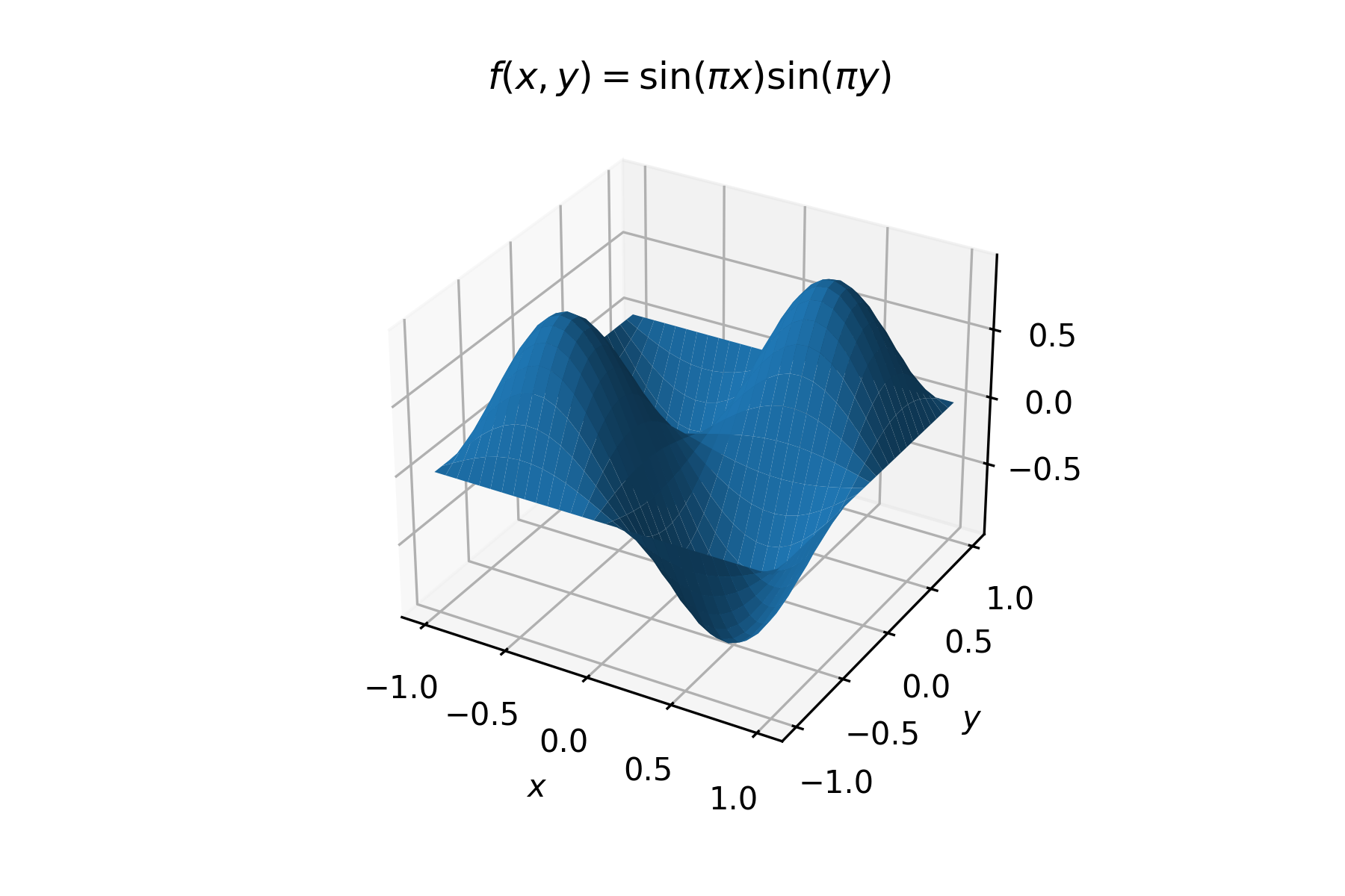
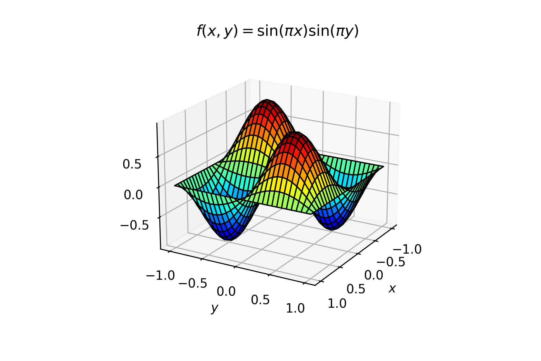
Lets produce a surface plot of the bi-variate function \(f(x, y) = \sin(\pi x) + \cos(\pi y)\) for \(x, y \in [-1, 1]\). Enter the following code into your program.
# Plot surface
x = np.linspace(-1, 1, 30)
y = np.linspace(-1, 1, 30)
X, Y = np.meshgrid(x, y)
Z = np.sin(np.pi * X) * np.sin(np.pi * Y)

from mpl_toolkits.mplot3d import Axes3D

fig = plt.figure()
ax = plt.axes(projection='3d')
ax.plot_surface(X, Y, Z)
plt.xlabel('$x$')
plt.ylabel('$y$')
plt.title('$f(x,y) = \sin(\pi x)\sin(\pi y)$')
plt.show()
Run your program and you should see the following plot added to the Plots pane.
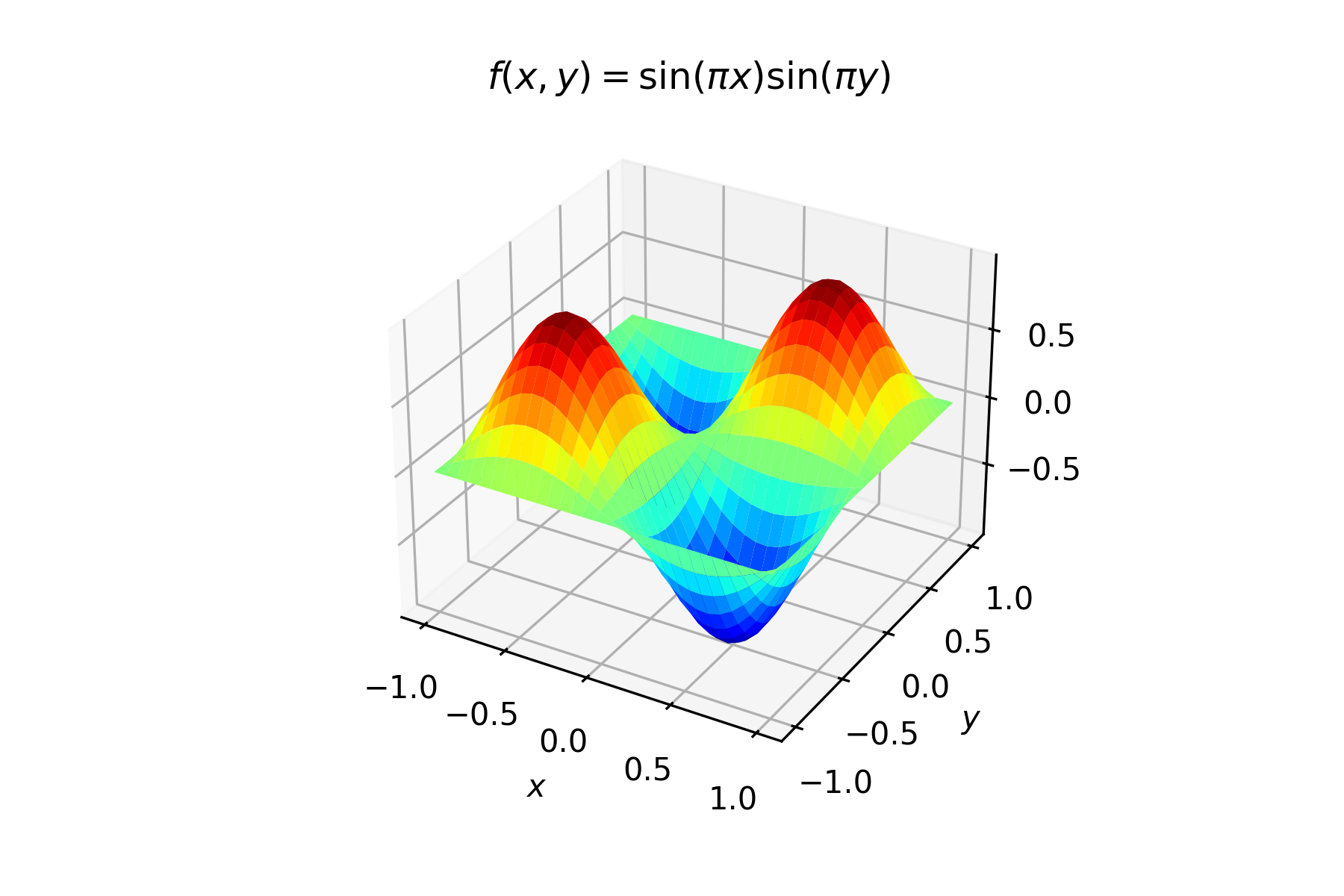
6.5.1. Colormaps#
The plot of the surface shown above uses the default maplotlib colour of blue which is pretty uninspiring. We can add colours to a surface plot in the form of a colormap where the color used for the surface is based on some value, e.g., the height. A colormap can be added to a surface plot using the cmap property
ax.plot_surface(X, Y, Z, cmap='colormap')
where colormap is the name of the colormap to be applied (see matplotlib documentation for a list of these). Lets demonstrate this by applying the jet colormap to our surface plot,change your code so that the plotting command looks like the following.
ax.plot_surface(X, Y, Z, cmap='jet')
Run your program and you should see the following plot added to the Plots pane.
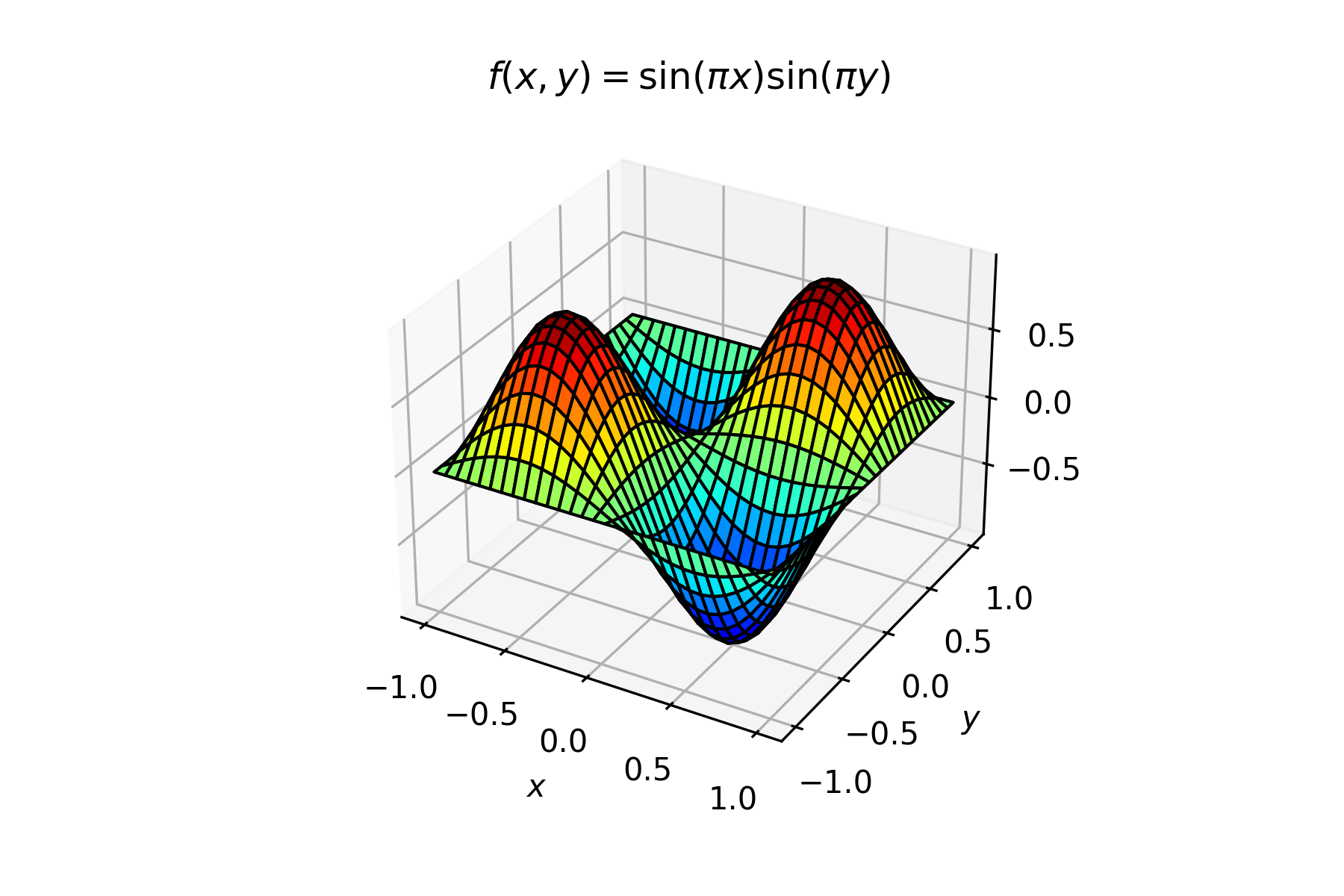
6.5.2. Line colour#
The default line colour for matplotlib surface plots is white which can make the detail of a surface difficult to see. The line colour can be changed using the edgecolor property
ax.plot_surface(X, Y, Z, edgecolor='colour')
Note that edgecolor can be abbreviated to ec. Let change the line colour of our surface plot to black, change your code so that the plotting command looks like the following.
ax.plot_surface(X, Y, Z, cmap='jet', edgecolor='k')
Run your program and you should see the following plot added to the Plots pane.
6.5.3. View angle#
With 3D plots we can control the position of the viewpoint using the view_init() function
ax.view_init(elev=elevation, azim=azimuth)
where elevation and azimuth are the angles (in degrees) that specify the vertical and horizontal position of the viewpoint relative to the centre of view.
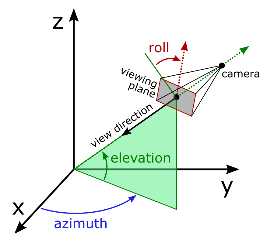
Fig. 6.7 Azimuth and elevation angles (from matplotlib.org)#
Lets view our surface plot from an azimuth angle of 30\(^\circ\) and an elevation of 20\(^\circ\). Enter the following code into your program.
# View angle
ax.view_init(elev=20, azim=30)
Run your program and you should see the following plot added to the Plots pane.
6.5.4. Exercise#
Exercise 6.7
Produce a surface plot of the function \(f(X, y) = \exp(-20((x - 0.5)^2 + (y - 0.5)^2))\) over the domain \(x,y \in [0, 1]\) using the autumn colormap.