13.6. Image plots#
Image plots (also known as raster plots) are plots which consist of an array of small squares called pixels. In Python image plots can be produced using the imshow() function.
imshow(img)
where img is a:
\(m\times n\) array of values;
\(m \times n \times 3\) array of RGB values which can either floating point values in the range \([0,1]\) or integer values in the range \([0,255]\).
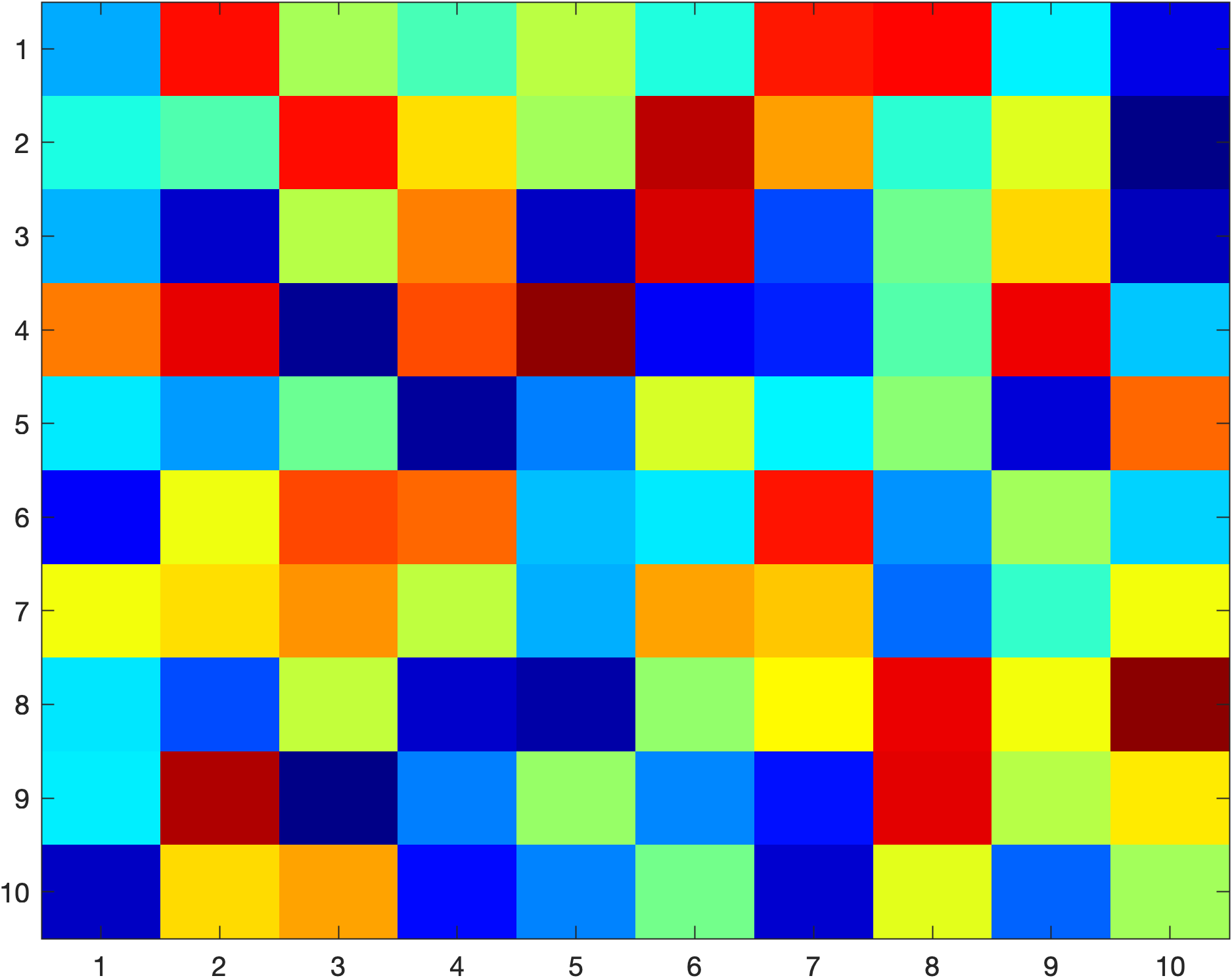
To demonstrate lets create an image plot using a \(10 \times 10\) array of random values in the range 0 to 255. Enter the following code into your program.
% Image plots
img = 255 * rand(10);
image(img)
Run your program and you should see the following plot added to the plot window.

Note that the vertical axis increments down from the top-left hand corner. This is because images use matrix indexing, so the index img(1,1) is the pixel in the top left corner.
13.6.1. Changing the aspect ratio#
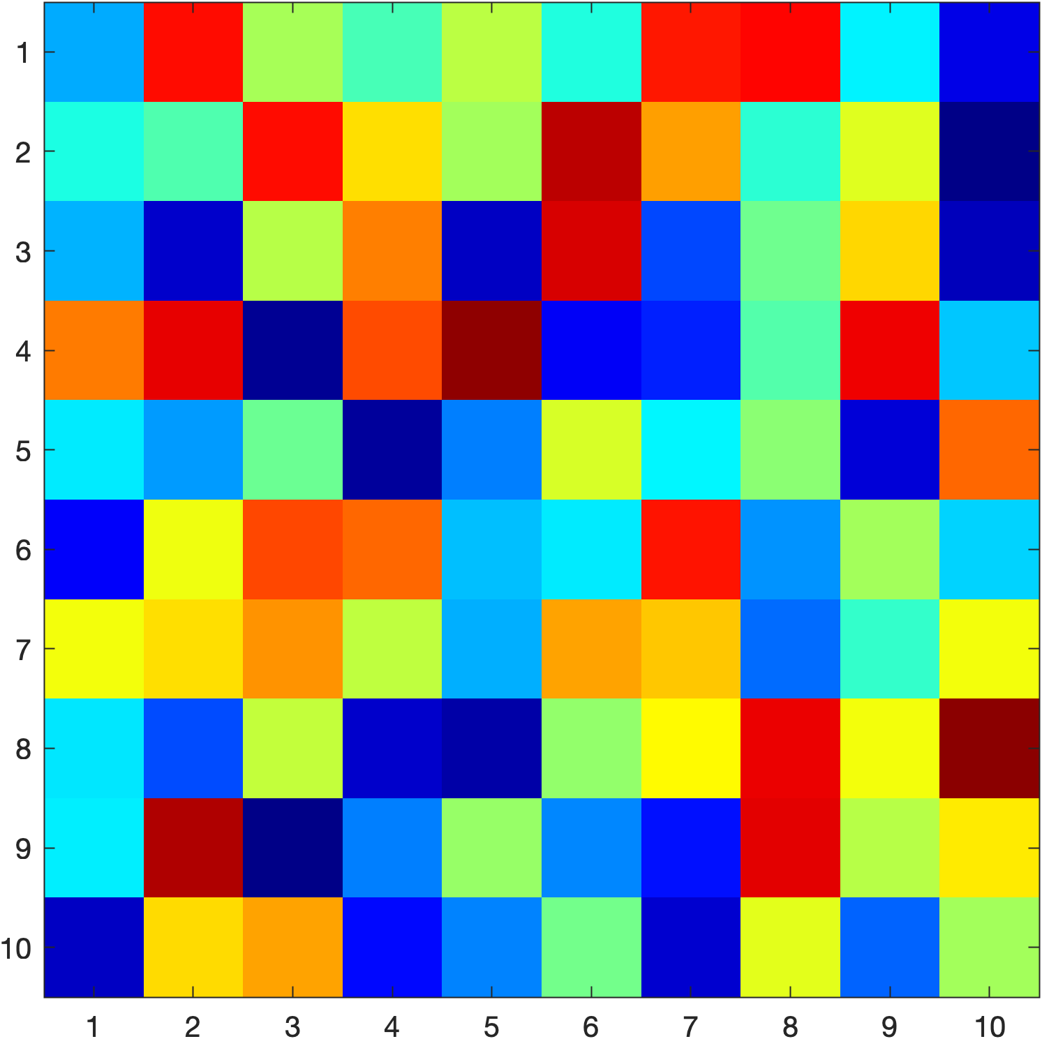
If you look carefully at the plot of the random values above you may notice that the pixels are not square. We can force the pixels to appear square (and therefore display images in the correct aspect ratio) by adding the following command to your program.
axis equal tight
Running your program again you should now see that the pixels are square

13.6.2. Reading an image file#
We can read in an image file into an \(m\times n \times 3\) array using the imread() function.
img = imread(filename)
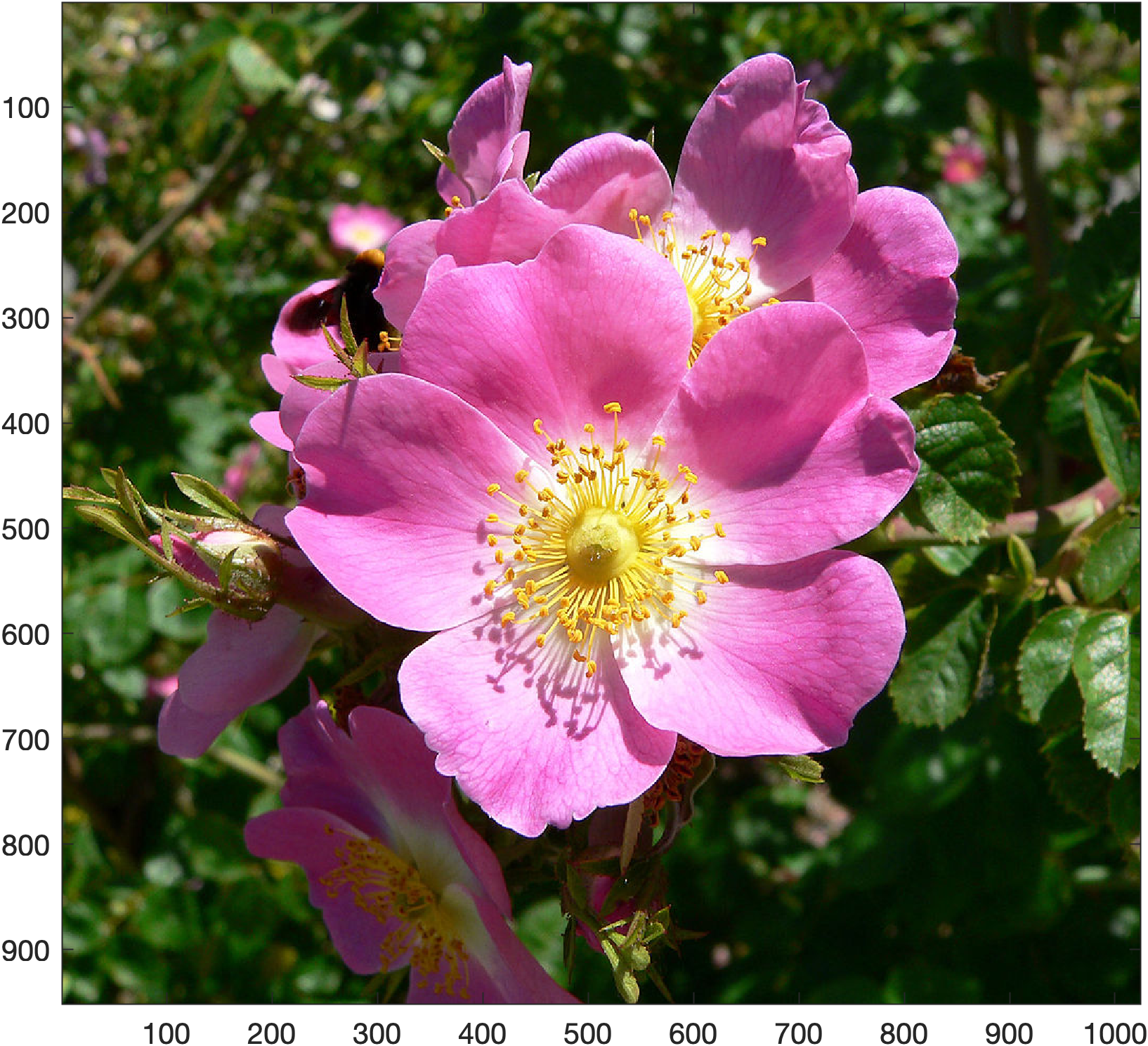
Where filename is the name of the image file. This allows us to perform image manipulation operations on the image. Lets demonstrate this by reading an image file, outputting its size and plotting the image. Download the image file flower.jpg to your OneDrive folder (in the same directory you use for these Python labs programs) and enter the following code into your program.
% Reading an image file
img = imread('flower.jpg');

% Determine the size of the image in pixels
[height, width, colours] = size(img);
fprintf('\nwidth       : %i\n', width)
fprintf('height      : %i\n', height)
fprintf('no. colours : %1i\n', colours)

% Plot the image
image(img)
axis equal tight
Run your program and you should see the following added to the command window
width       : 1024
height      : 951
no. colours : 3
Here the image is 1024 pixels wide by 951 pixels tall and each pixel consists of a combination of 3 colour values. As well as this command window output the following plot added to the plot window.

13.6.3. Image processing#
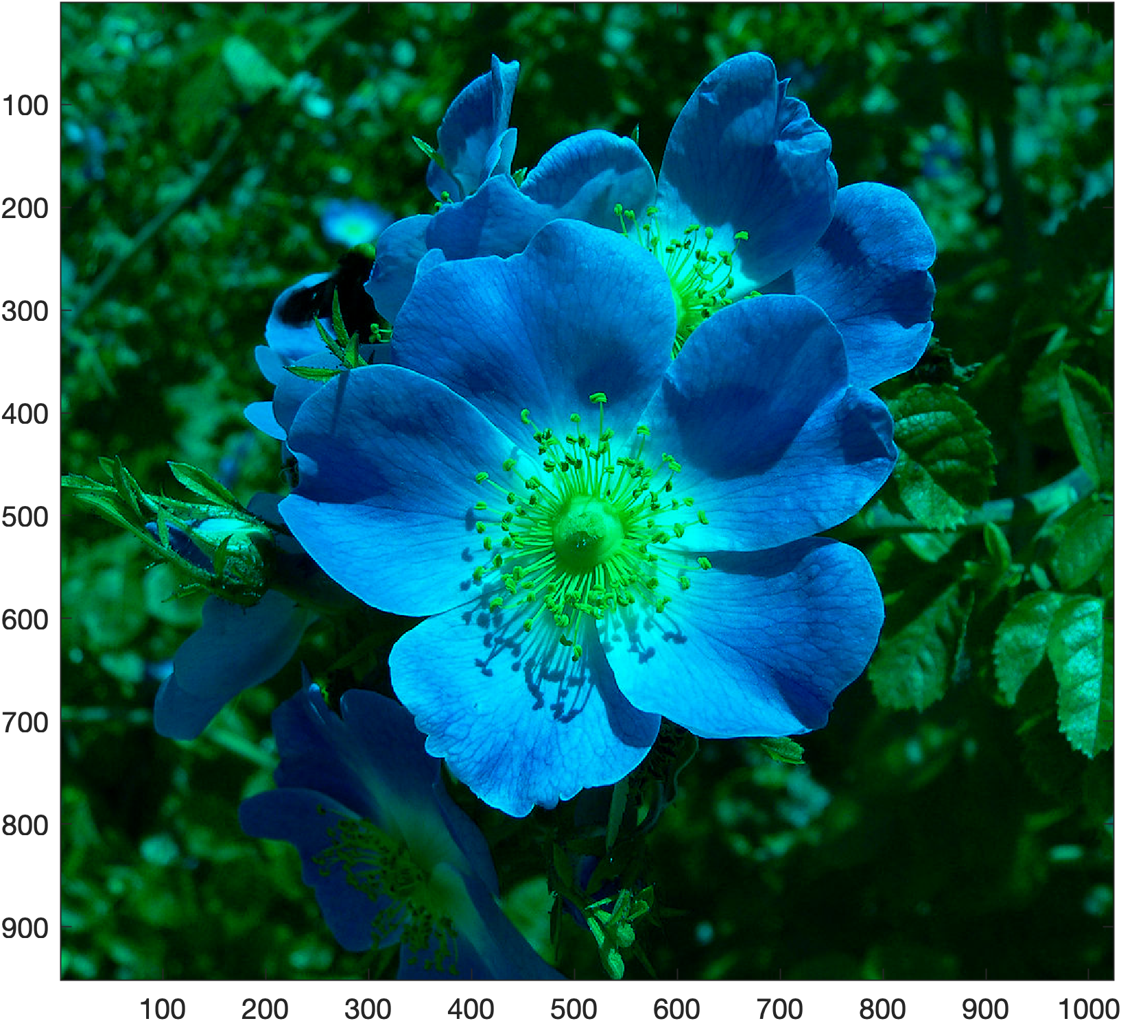
Once an image has been read into MATLAB we can apply image processing techniques to change the colour values of particular pixels. To demonstrate this lets remove all red values from the image of the flower. We have seen that the img array is a \(951 \times 1024 \times 3\) array and the 3 colour levels represent values of red, green and blue colours respectively (think of a building where each pixel is a room on a floor and each floor is a colour level). So to remove the red values we can set all of the values of the first level to zero. Enter the following code into your program.
% Image processing
img2 = img;
img2(:,:,1) = 0;
image(img2)
axis equal tight
Here we have made a copy of the original image using the np.copy() function and assigned it the name img2. Then we set all values in the first colour level to 0 before plotting the altered image. Run your program and you should see the following plot added to the plot window.

13.6.4. Exercises#
Exercise 13.9
Generate a \(21 \times 21\) array where the value of the element is calculated using
Plot the image of your array applying the jet colormap.
Exercise 13.10
Download the image file Dalton_building.jpg and save it to the same folder you use for your programming skills labs. Determine the number of pixels in the image and plot the image.
Exercise 13.11
A colour image can be converted to grayscale by setting the red, green and blue colour values equal to the weighted sum based on the average persons relative perception of the brightness of red, green and blue light which is
Convert the image from Exercise 13.10 into grayscale and plot it.