13.3. Scatter plots

Scatter plots can be produced using the scatter() function.

scatter(x, y, Linespec)

Where x and y are one-dimensional co-ordinate arrays and colour and Linespec are characters specifying the colour and marker used for each point (see Table 13.1).

To demonstrate this enter the following code into your program.

% Scatter plots
x = rand(1, 100);
y = rand(1, 100);

clf
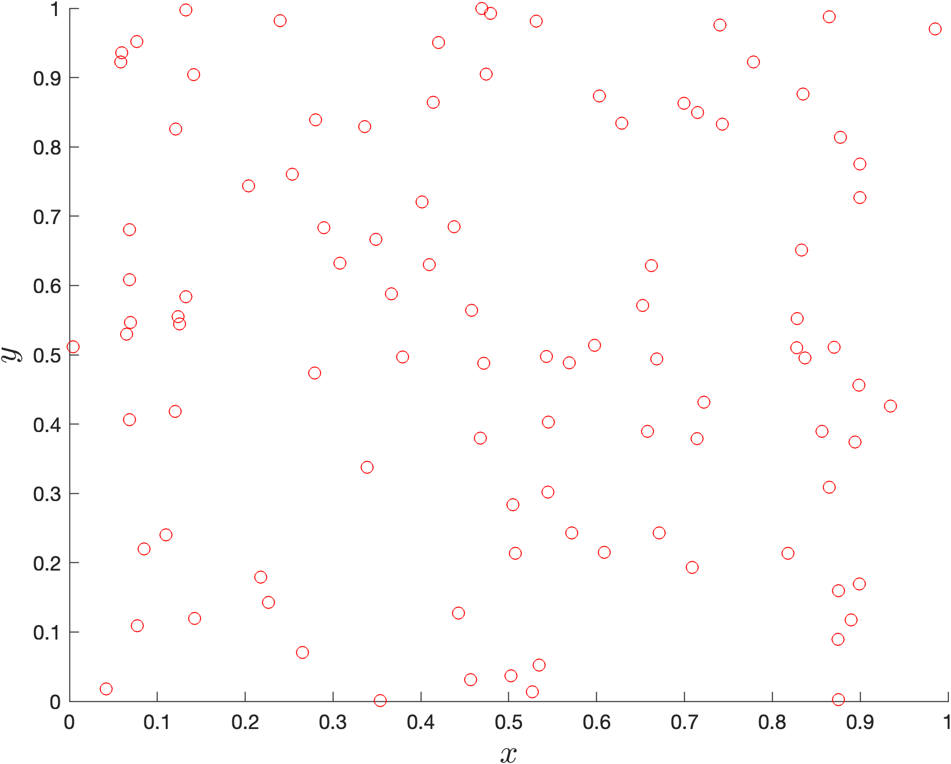
scatter(x, y, 'r')
xlabel('$x$', FontSize=16, Interpreter='latex')
ylabel('$y$', FontSize=16, Interpreter='latex')

The rand(1, 100) function generates an array of 100 random numbers in the range \([0, 1]\). Run your program and you should see the following plot added to the plot window (note that yours will look slightly different to this one due to the random numbers generated).

---

13.3.1. Exercises

Exercise 13.5

Produce a scatter plot using the arrays x and y given below. Format your plot so that the points are plotted using blue diamonds and the axes are scaled so that \(x,y \in [0, 1]\).

x = np.array([ 0.1734, 0.3909, 0.8314, 0.8034, 0.0605, 0.3993, 0.5269, 0.4168, 0.6569, 0.6280 ])
y = np.array([ 0.0717, 0.1665, 0.7881, 0.5486, 0.0702, 0.2382, 0.3031, 0.2341, 0.4335, 0.4265 ])

Exercise 13.6

We can calculate a line of bets fit for the data from Exercise 13.5 using a linear regression model \(y = mx + c\) where \(m\) is the slope of the line and \(c\) is the \(y\)-intercept. To compute \(m\) and \(c\) we can rewrite the linear model as \(\vec{y} = A\vec{p}\) where \(\vec{y} = (y_1, y_2, \ldots, y_n)^\mathsf{T}\), \(\vec{p} = (m, c)^\mathsf{T}\) and

\[\begin{split} \begin{align*} A= \begin{pmatrix} x_1 & 1 \\ x_2 & 1 \\ \vdots & \vdots \\ x_n & 1 \end{pmatrix}. \end{align*} \end{split}\]

We then solve for \(m\) and \(c\) using the NumPy command line = A \ y' which calculates the least squares solution where line = [m, c] which minimises the difference between the points \((x_i,y_i)\) and the line \(y=mx+c\).

Calculate the line of best fit for the data from Exercise 13.5 and add it to your scatter plot.