13.5. Contour plots#
Contour plots show points of equal value can be produced using the contour() function.
contour(X, Y, Z)
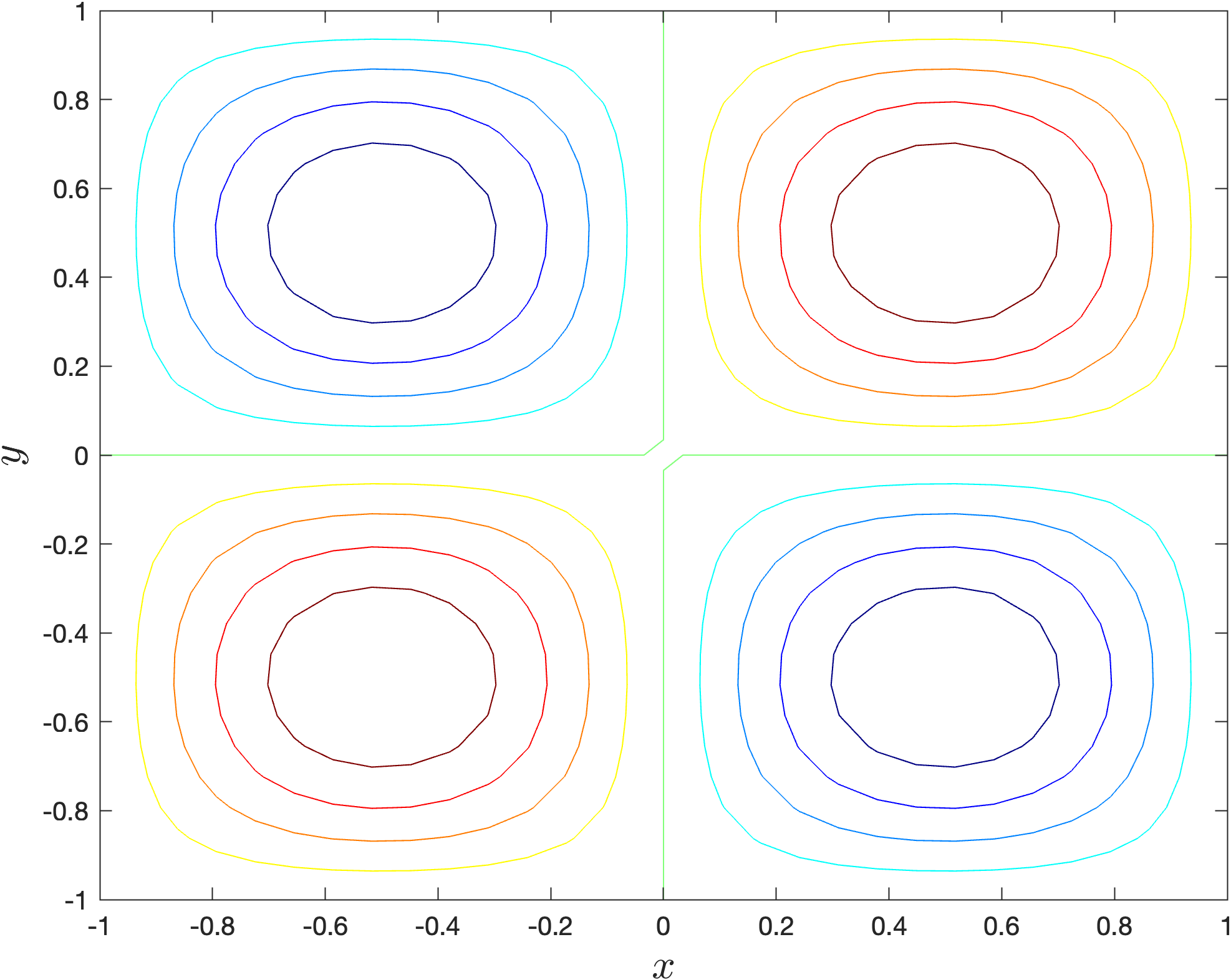
where X, Y and Z are 2D co-ordinate arrays. Lets create a contour plot of the bi-variate function \(f(x, y) = \sin(\pi x)\sin(\pi y)\) that we used in the previous section on surface plots. Enter the following code into your program.
% Contour plots
clf
contour(X, Y, Z)
xlabel('$x$', FontSize=16, Interpreter='latex')
ylabel('$y$', FontSize=16, Interpreter='latex')
Run your program and you should see the following plot added to the plot window.

13.5.1. Contour levels#
The number of contour lines that are used a draw a contour plot can be specified in the contour() function.
contour(X, Y, Z, levels)
where levels is an integer. To demonstrate this enter the following code into your program before the show() function.
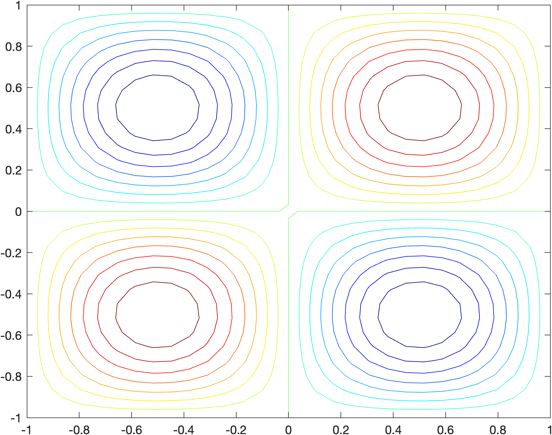
contour(X, Y, Z, 15)
Here we specify that we want 15 contour lines on our contour plot. Run your program and you should see the following added to the Plots pane.

13.5.2. Contour labels#
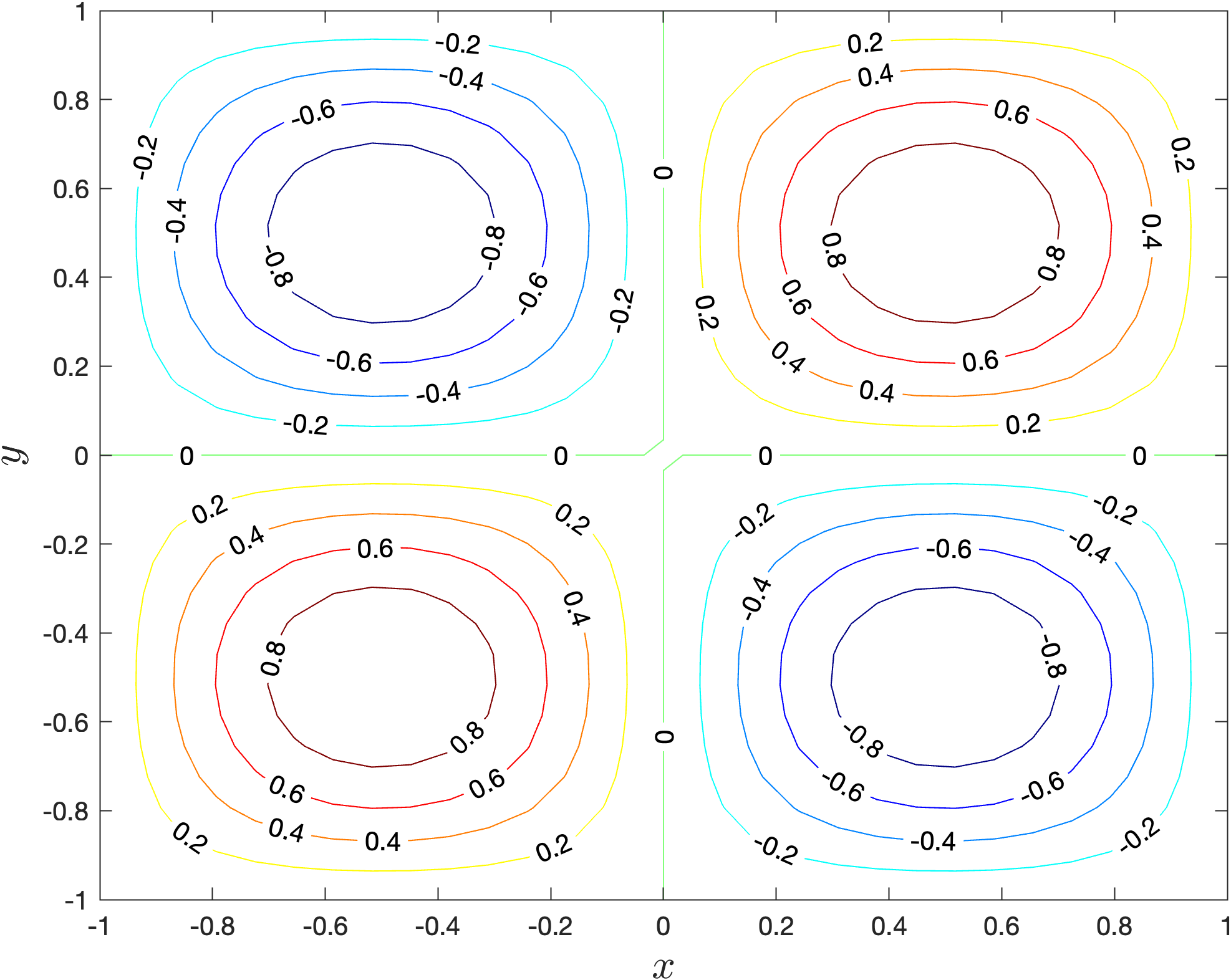
Looking at our contour plots it may be difficult to see which contour lines represent the higher values. To help with this we can add labels to each of our contour lines using the clabel() function.
[C, h] = contour(X, Y, Z)
clabel(C, h)
To demonstrate this enter the following code into your program.
% Contour labels
clf
[C,h] = contour(X, Y, Z)
clabel(C, h)
xlabel('$x$', FontSize=16, Interpreter='latex')
ylabel('$y$', FontSize=16, Interpreter='latex')
Run your program and you should see the following plot added to the plot window.

13.5.3. Exercise#
Exercise 13.8
Produce a contour plot of the function \(z=(z_1-z_2)^2\) where \(z_1=\exp(-x^2-y^2)\) and \(z_2=\exp(-(x-1)^2-(y-1)^2)\) over the domain \(x,y\in[-2,3]\).