9. Normal Mapping#
In the last lab on lighting we saw that the diffuse and specular reflection models used the normal vector to determine the fragment colour. The vertex shader was used to interpolate the normal vectors for each fragment based on the normal vectors at the vertices of a triangle. This works well for smooth objects, but for objects with a rough or patterned surface we don’t get the benefits of highlights and shadow. Normal mapping is technique that uses a texture map to define the normal vectors for each fragment so that when a lighting model is applied it gives the appearance of a non-flat surface.

Fig. 9.1 Normal mapping applies a texture of normals for each fragment giving the appearance of a non-flat surface.#
A normal map is a texture where the RGB colour values of each textel is used for the normal vector \(\mathbf{n} = (n_x, n_y, n_z)\) where \(n_x\), \(n_y\) and \(n_z\) values are determined by the red, green and blue colours values respectively (Fig. 9.2).

Fig. 9.2 The RBG values of a normal map give the values of the normal vectors.#
Note that since the OpenGL co-ordinate system has the \(z\)-axis pointing outwards towards the viewer then normal maps take on a mostly blue appearance.
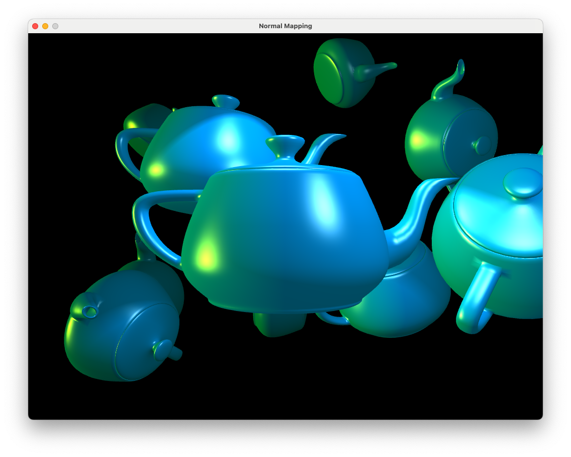
Compile and run the project \(Lab09_Normal_maps\) and you will see that we have the scene used at the end of last lab on Lighting with the teapots lit using two point lights, a spotlight and a directional light.
A Light class has been created to handle the light sources. Take a look at the light.hpp and light.cpp files and you will see the following Light class methods
addPointLight(),addSpotLight(),addDirLight()- these are used to add another light source to the scenetoShader()- sends all of the lighting uniforms to the shaderdraw()- draws the light source
9.1. Tangent space#
We have already seen in 6. 3D worlds that we can use transformations to map co-ordinates and vectors between the model, view and screen spaces. To apply normal mapping we need to perform our lighting calculations in a new space called the tangent space. The tangent space is a 3D space where vectors are defined in terms of three vectors: tangent, bitangent and normal vectors (Fig. 9.3).

Fig. 9.3 Normal, tangent and the bitangent vectors.#
Normal vector, \(\mathbf{n}\) - we have already met the normal vector which is a vector perpendicular to the surface
Tangent vector, \(\mathbf{t}\) - this is a vector that points along the surface so is perpendicular to the normal vector
Bitangent vector, \(\mathbf{b}\) - this is a vector that is perpendicular to both the normal and tangent vectors
There are an infinite number of vectors on a plane that is perpendicular to the normal vector so we have a choice for the tangent and bitangent vectors. A natural choice is to use vectors that point along the edges of the normal map, we know these are perpendicular and this also means we are consistent for neighbouring triangles.

Fig. 9.4 The tangent space is defined by the tangent, bitangent and normal vectors.#
The tangent and bitangent vectors are calculated using the model space vertex co-ordinates of the triangle \((x_0,y_0,z_0)\), \((x_1,y_1,z_1)\) and \((x_2,y_2,z_2)\) and their corresponding texture co-ordinates \((u_0,v_0)\), \((u_1,v_1)\) and \((u_2,v_2)\).

Fig. 9.5 The tangent, \(\mathbf{t}\), and bitangent, \(\mathbf{b}\), vectors are calculated by mapping the model space triangle onto the normal map space.#
We first calculate vectors that point along two sides of the triangle in the model space
and calculate the difference in the \((u,v)\) co-ordinates for these edges
The tangent, \(\mathbf{t}\), and bitangent, \(\mathbf{b}\), vectors can then be calculated using
To see the derivation of these equations click on the dropdown below.
Calculating the tangent and bitangent vectors
Consider Fig. 9.5 where a triangle is mapped onto the normal map using texture co-ordinates \((u_0,v_0)\), \((u_1,v_1)\) and \((u_2,v_2)\). If the vectors \(\mathbf{t}\) and \(\mathbf{b}\) point in the co-ordinate directions of the normal map then the tangle space positions along the triangle edges \(E_1\) and \(E_2\) can be calculated using
where \(\Delta u_1 = u_1 - u_0\), \(\Delta v_1 = v_1 - v_0\), \(\Delta u_2 = u_2 - u_1\) and \(\Delta v_2 = v_2 - v_1\). We can express this using matrices
We want to calculate \(\mathbf{t}\) and \(\mathbf{b}\) and we know the values of \(E_1\), \(E_2\), \(\Delta u_1\), \(\Delta v_1\), \(\Delta u_2\) and \(\Delta v_2\). Using the inverse of the square matrix we can rewrite this equation as
Writing the out for the \(\mathbf{t}\) and \(\mathbf{b}\) vectors we have
Once we have the tangent, bitangent and normal vectors we can form a matrix that transforms from the tangent space to an arbitrary space (e.g., the view space). The matrix that achieves this a 3 \(\times\) 3 matrix known as the \(TBN\) matrix
where \(\mathbf{t} = (t_x, t_y, t_z)\), \(\mathbf{b} = (b_x, b_y, b_z)\) and \(\mathbf{n} = (n_x, n_y, n_z)\). We will be performing our lighting calculations in the tangent space so we want to transform from the view space to the tangent space. To do this we calculate the inverse of the \(TBN\) matrix. Fortunately this is an orthogonal matrix where the inverse is simply the transpose, i.e., \(TBN^{-1} = TBN^\mathsf{T}\), which is an easy calculation.
9.1.1. Calculating the tangent and bitangent vectors#
All of the lighting calculations are performed by the shaders so we calculate the tangent and bitangent vectors in our C++ program and pass them to the vertex shader using uniforms. The model class contains all of the attributes for a model so we create two vectors that will contain the tangents and bitangents for each of the vertices of the model. In the model.hpp file add the following code after we have declared a vector array for the normals.
std::vector<glm::vec3> tangents;
std::vector<glm::vec3> bitangents;
We are going to send the tangents and bitangents to the GPU using vertex buffers in the same way as we did for the vertices, texture co-ordinates and normal vectors. Under the private: declaration add the identifiers for the tangent and bitangent buffers.
unsigned int tangentBuffer;
unsigned int bitangentBuffer;
We now create a private method for our model class to calculate the tangent and bitangent vectors. Add the following method declaration.
 // Calculate tangents and bitangents
 void calculateTangents();
Then in the model.cpp file we define the calculateTangents() method.
void Model::calculateTangents()
{
    for (unsigned int i = 0; i < vertices.size(); i += 3)
    {
        // Calculate edge vectors and deltas
        glm::vec3 E1  = vertices[i+1] - vertices[i];
        glm::vec3 E2  = vertices[i+2] - vertices[i+1];
        float deltaU1 = uvs[i+1].x - uvs[i].x;
        float deltaV1 = uvs[i+1].y - uvs[i].y;
        float deltaU2 = uvs[i+2].x - uvs[i+1].x;
        float deltaV2 = uvs[i+2].y - uvs[i+1].y;

        // Calculate tangents
        float denom         = 1.0f / (deltaU1 * deltaV2 - deltaU2 * deltaV1);
        glm::vec3 tangent   = (deltaV2 * E1 - deltaV1 * E2) * denom;
        glm::vec3 bitangent = (deltaU1 * E2 - deltaU2 * E1) * denom;

        // Set the same tangents for the three vertices of the triangle
        tangents.push_back(tangent);
        tangents.push_back(tangent);
        tangents.push_back(tangent);
        bitangents.push_back(bitangent);
        bitangents.push_back(bitangent);
        bitangents.push_back(bitangent);
    }
}
This code calculates the tangent and bitangent vectors using equation (9.1) and adds them the tangents and bitangents vectors. We want these to be calculated whenever we create a model so amend the Model class constructor at the top of the file and add the following before setupBuffers() is called.
// Calculate tangent and bitangent vectors
calculateTangents();
The last addition we need to make to the Model class is to setup the buffers for the tangent and bitangent and copy these across to the GPU. Add the following to the setupBuffers() method (before we unbind the VAO).
// Create tangent buffer
GLuint tangentBuffer;
glGenBuffers(1, &tangentBuffer);
glBindBuffer(GL_ARRAY_BUFFER, tangentBuffer);
glBufferData(GL_ARRAY_BUFFER, tangents.size() * sizeof(glm::vec3), &tangents[0], GL_STATIC_DRAW);

// Create bitangent buffer
GLuint bitangentBuffer;
glGenBuffers(1, &bitangentBuffer);
glBindBuffer(GL_ARRAY_BUFFER, bitangentBuffer);
glBufferData(GL_ARRAY_BUFFER, bitangents.size() * sizeof(glm::vec3), &bitangents[0], GL_STATIC_DRAW);

// Bind the tangent buffer
glEnableVertexAttribArray(3);
glBindBuffer(GL_ARRAY_BUFFER, tangentBuffer);
glVertexAttribPointer(3, 3, GL_FLOAT, GL_FALSE, 0, (void*)0);

// Bind the bitangent buffer
glEnableVertexAttribArray(4);
glBindBuffer(GL_ARRAY_BUFFER, bitangentBuffer);
glVertexAttribPointer(4, 3, GL_FLOAT, GL_FALSE, 0, (void*)0);
These are essentially the same as what we’ve done previously for the vertices, texture co-ordinates and normal vectors. Note that the tangent and bitangent buffers are bound to attributes 3 and 4 respectively.
9.2. Shaders#
9.2.1. Vertex shader#
In the vertex shader we need to calculate the tangent space fragment position, light position and light direction. We could do this in the fragment shader but since that is called for each fragment in the triangle and the vertex shader is just called 3 times per triangle it is much more efficient to do it in the vertex shader.
The first change we need to make to the vertex shader is to declare the new tangent and bitangent inputs. These were bound to attributes 3 and 4 respectively so edit your file so that we input the tangets and bitangent buffers.
layout(location = 3) in vec3 tangent;
layout(location = 4) in vec3 bitangent;
We need to transform the fragment position, light position and direction vector to the tangent space and to do so we calculate the \(TBN\) matrix. Before the view space fragment position and normal vector are calculated add the following code.
// Calculate the TBN matrix that transforms view space to tangent space
mat3 invMV = transpose(inverse(mat3(MV)));
vec3 t     = normalize(invMV * tangent);
vec3 b     = normalize(invMV * bitangent);
vec3 n     = normalize(invMV * normal);
mat3 TBN   = transpose(mat3(t, b, n));
Here we transform the tangent, bitangent and normal vectors to the view space using the matrix from equation (8.3) which are then used to calculate the \(TBN\) matrix. Remember that by transposing the \(TBN\) matrix we are calculating its inverse so here the TBN matrix will transform from the view space to the tangent space.
Note
Some people transform the vectors to the world space instead of the view space, however, this means that we need to also calculate the tangent space position of the camera for the eye vector calculation in the fragment shader. Doing this would mean we have additional uniforms and vector calculations. Since the camera position in the view space is \((0,0,0)\) then it is also \((0,0,0)\) in the tangent space so by transforming the vectors to the view space we don’t need to worry about this.
We also have to calculate the tangent space fragment position, light position and direction vector using the \(TBN\) matrix. Since we have multiple light sources we need to output an array of vectors for the position and direction of each light source. Add the following to the outputs of the vertex shader
out vec3 tangentSpaceLightPosition[maxLights];
out vec3 tangentSpaceLightDirection[maxLights];
Then replace the code used to calculate the view space vectors with the following code.
// Output tangent space fragment position, light positions and directions
fragmentPosition = TBN * vec3(MV * vec4(position, 1.0));
for (int i = 0; i < maxLights; i++)
{
    tangentSpaceLightPosition[i]  = TBN * lightSources[i].position;
    tangentSpaceLightDirection[i] = TBN * lightSources[i].direction;
}
9.2.2. Fragment shader#
Now that we have transformed the vectors to the tangent space in the vertex shader we need to make a few changes to the fragment shader. The beauty of the tangent space is that it is orthogonal so we don’t need to change any of our lighting calculations. This means we only need to make a few changes to the fragment shader.
First, declare the inputs for the array of tangent space light source position and direction
in vec3 tangentSpaceLightPosition[maxLights];
in vec3 tangentSpaceLightDirection[maxLights];
We have an additional texture for the normal map so we use a sampler uniform. Add the following where we declared the diffuse map uniform.
uniform sampler2D normalMap;
Within the main function we obtain the normal vector from the normal map. Since the values in a texture are between 0 and 1 and we need the values of a normal vector to be between -1 and 1 we scale using the following
Before the main() function add the following code
// Get the normal vector from the normal map
vec3 Normal = normalize(2.0 * vec3(texture(normalMap, UV)) - 1.0);
Then in the Lab09_Normal_maps.cpp file add the normal map texture to the teapot object where we added the diffuse map.
teapot.addTexture("../objects/diamond_normal.png", "normal");
Compile and run the program and you should see the following.

Fig. 9.6 Normal map applied to teapot objects.#
The surfaces of the teapots which are smooth now have the appearance of bumpy diamond plate simply by getting the normal vectors from a texture and performing the lighting calculations in the tangent space. Fig. 9.7 shows a closeup of the surface so we can see the detail.
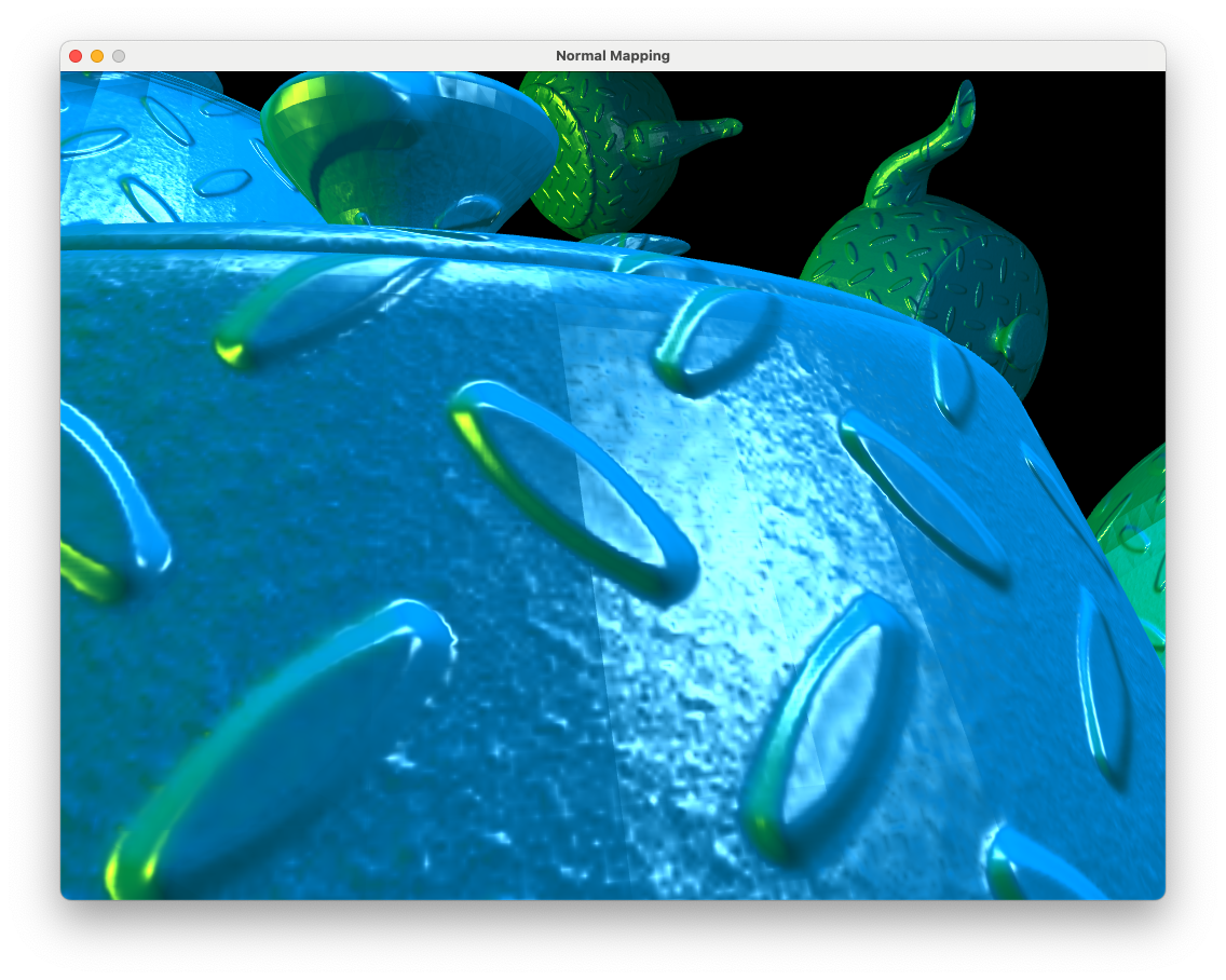
Fig. 9.7 Close up of the normal map applied to teapot objects.#
9.3. Re-orthogonalising the tangent space vectors#
In the close up view of the normal mapped teapot in Fig. 9.7 we can see a distinct line in the specular highlights where polygons that form the surface of the teapot join. The reason for this is that the tangent vector is not exactly perpendicular to the normal vector.
When a vertex is shared by multiple triangles the 3D modelling software (e.g., Blender) calculates a single normal vector for the vertex by averaging of the normal vectors for the triangles (Fig. 9.8). This saves memory and ensures that there is a smooth transition between the normal vectors across the surface.

Fig. 9.8 The vertex normal is the average of the normal of the triangles sharing that vertex.#
A problem with this is that when using a normal map we assume that the vertex normals are perpendicular to the triangle we are rendering. Since this is not the case so calculating the tangents and bitangents using equation (9.1) will not give an orthogonal set of vectors. We can get around this problem by re-orthogonalising the three vectors by adjusting the tangent vector a bit so that it is orthongonal to the normal vector.

Fig. 9.9 Re-orthogonalising T using the Gram-Schmidt process.#
Consider Fig. 9.9 where the tangent vector \(\mathbf{t}\) is non-orthogonal to the normal vector \(\mathbf{n}\). If \(\mathbf{n}\) and \(\mathbf{t}\) are unit vectors then if we subtract \((\mathbf{t} \cdot \mathbf{n}) \mathbf{n}\) from \(\mathbf{t}\) then this creates a vector \(\mathbf{t}_{new}\) that is orthogonal to \(\mathbf{n}\) (this is known as the Gram-Schmidt process). We can use the cross product between \(\mathbf{n}\) and \(\mathbf{t}\) to calculate the bitangent vector \(\mathbf{n}\).
Edit the vertex shader so that we re-orthogonalise \(\mathbf{t}\) and \(\mathbf{b}\).
// Calculate the TBN matrix that transforms view space to tangent space
mat3 invMV = transpose(inverse(mat3(MV)));
vec3 t     = normalize(invMV * tangent);
vec3 n     = normalize(invMV * normal);
t          = normalize(t - dot(t, n) * n);
vec3 b     = cross(n, t);
mat3 TBN   = transpose(mat3(t, b, n));
Compile and run the code once against and you should see a screen similar to the one below.
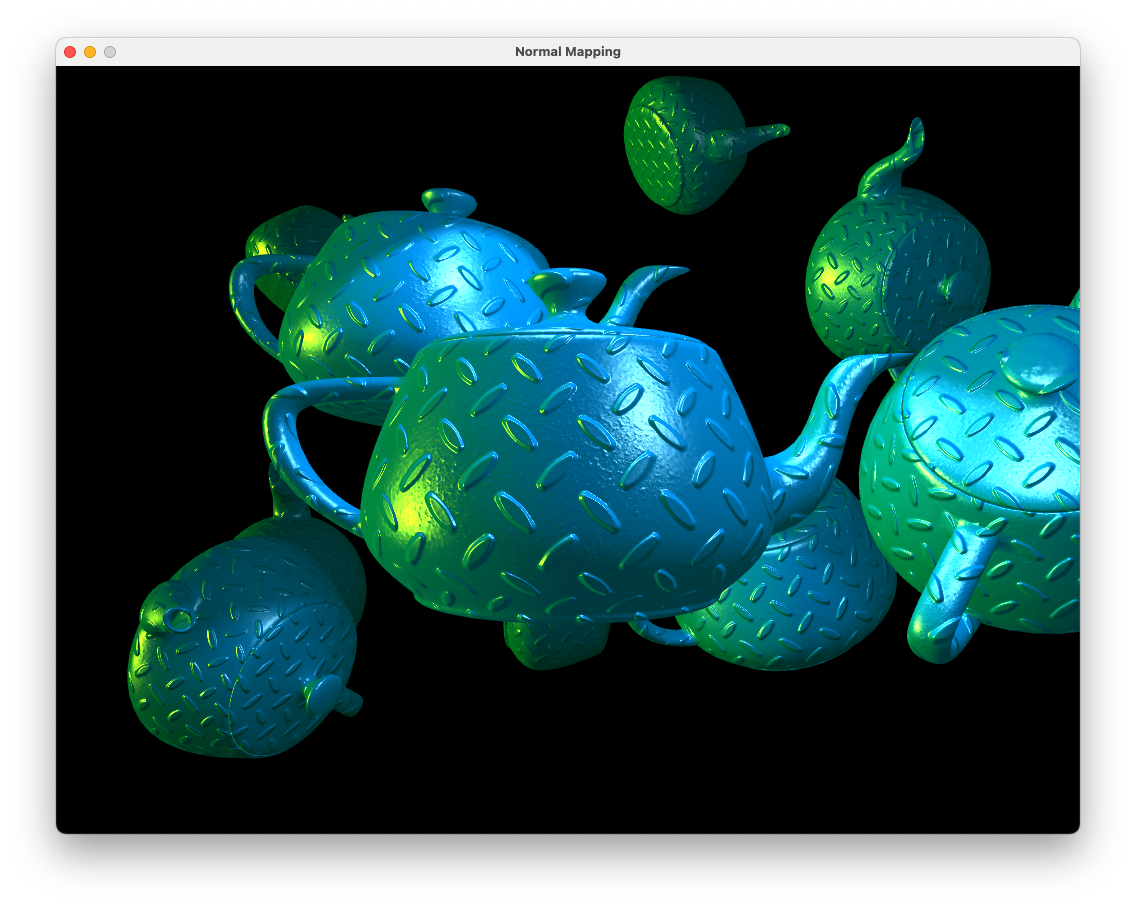
Fig. 9.10 A normal map with orthogonalised tangent and bitangent vectors.#
Now our tangent space vectors are orthogonal and we have a correct normal map applied.
9.4. Specular maps#
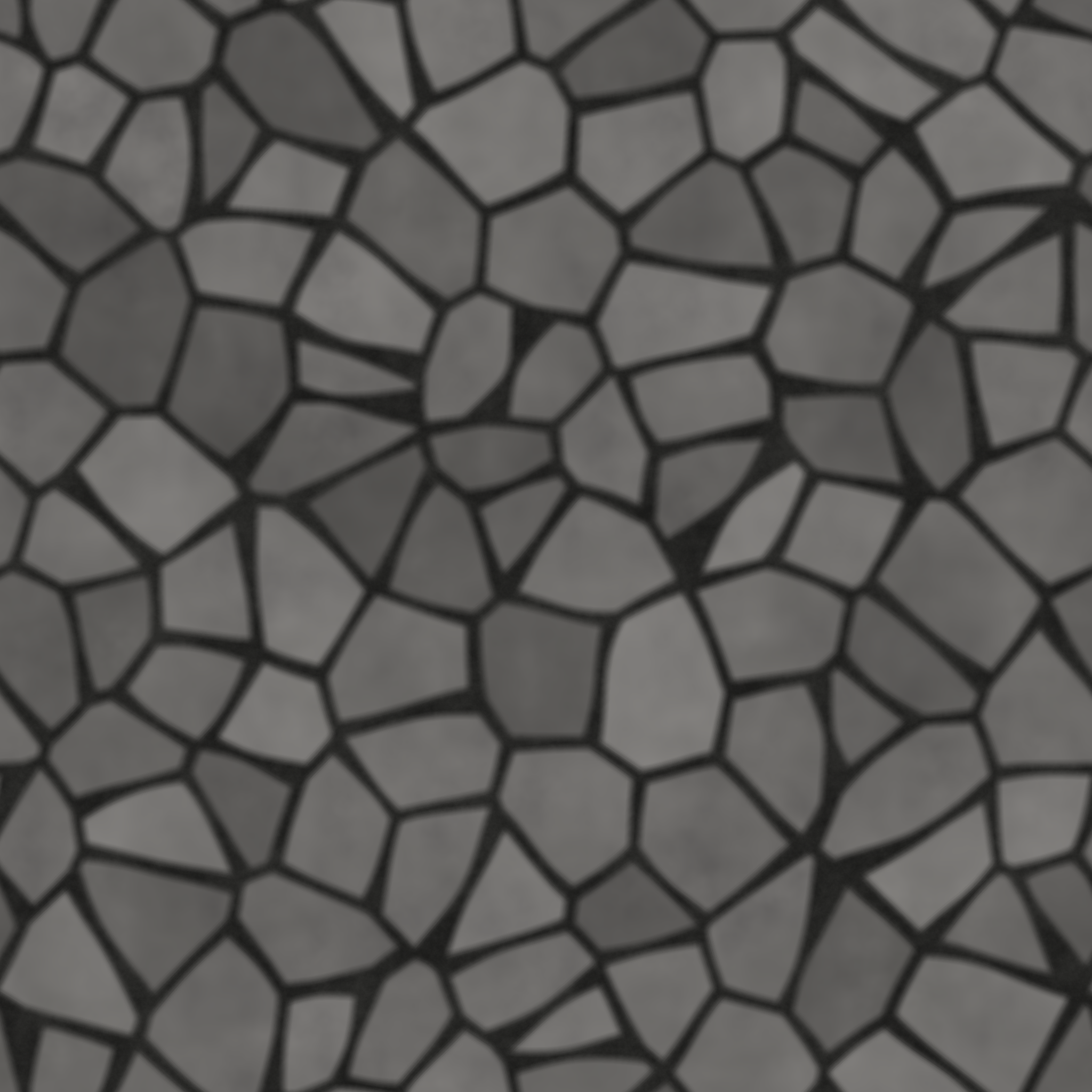
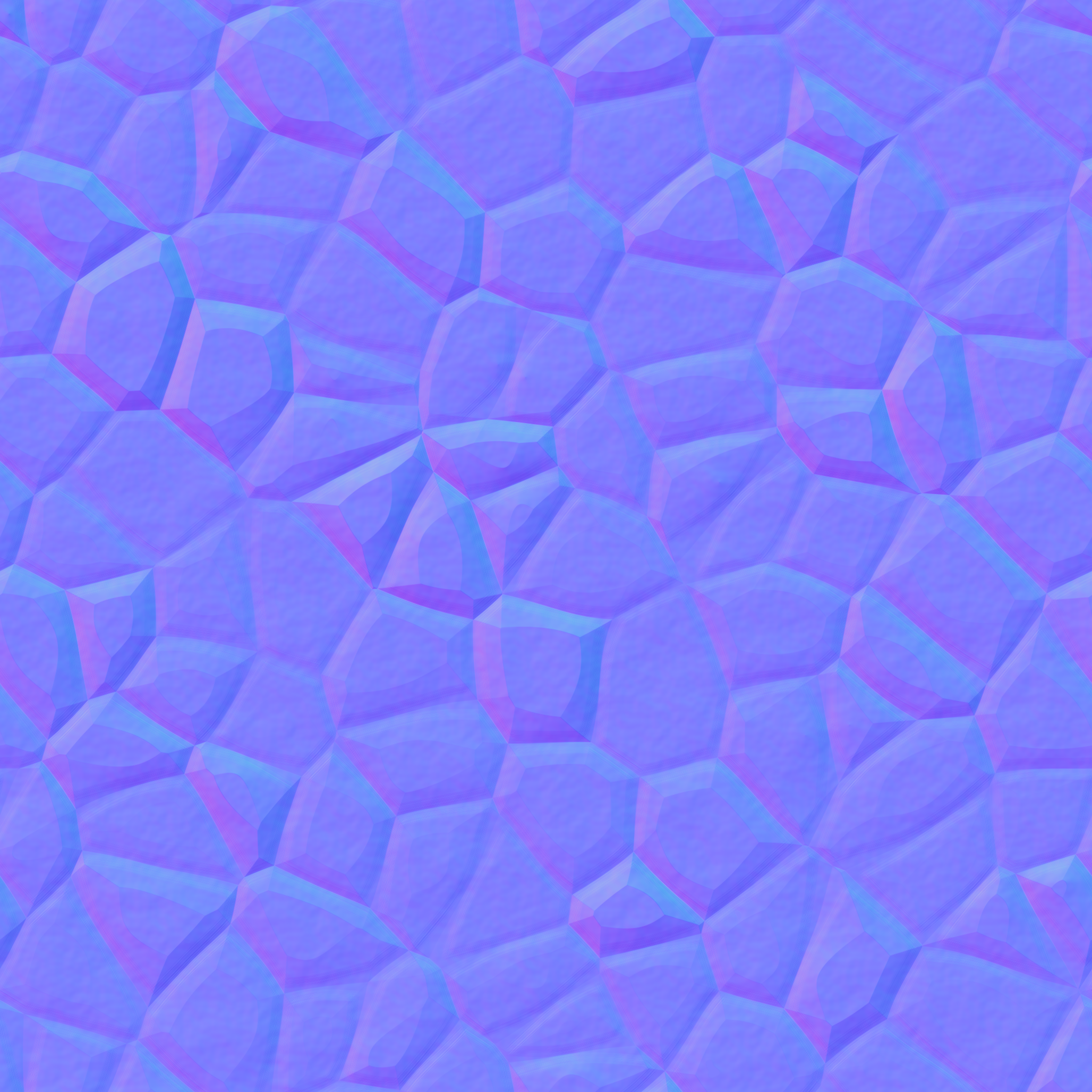
In addition to diffuse (texture) and normal maps we can also apply a specular map which can be used to control the specular highlights across a surface. Lets say we want to add a stone floor to our scene. We can add a horizontal polygon object for the floor and use a texture map Fig. 9.11 to give the impression of stones and a normal map Fig. 9.12 so that the stones are lit by the light sources.
To apply our stone floor we are going to have a different object than our old friend the teapot. We will also want to add multiple different objects in the future so it we are going to use a data structure to contain the world space position, rotation and scaling of our objects and then store this in a vector. Add the following code to the main.cpp file before the main() function.
// Data structures
struct Object
{
    glm::vec3 position = glm::vec3(0.0f, 0.0f, 0.0f);
    glm::vec3 rotation = glm::vec3(0.0f, 1.0f, 0.0f);
    glm::vec3 scale = glm::vec3(1.0f, 1.0f, 1.0f);
    float angle = 0.0f;
    float ka = 0.2f;
    float kd = 0.7f;
    float ks = 1.0f;
    float Ns = 20.0f;
    std::string name;
};
When we create an Object data structure the objects will have a default position at (0,0,0), the rotation and scale are unchanged and the object lighting properties are the same as what we have using so far (we can change these later if we want). Load the floor model and give it diffuse and normal textures where we load the teapot and lightModel models.
// Load models
Model teapot("../objects/teapot.obj");
Model lightModel("../objects/sphere.obj");
Model floor("../objects/flat_plane.obj");

// Add textures to models
teapot.addTexture("../objects/blue_diffuse.bmp", "diffuse");
teapot.addTexture("../objects/diamond_normal.png", "normal");
floor.addTexture("../objects/stones_diffuse.png", "diffuse");
floor.addTexture("../objects/stones_normal.png", "normal");
We are going to create a vector to contain the different objects. Add the following code after we have added the textures to the models.
// Define objects
std::vector<Object> objects;
Object object;
object.name = "teapot";
objects.push_back(object);

object.name = "floor";
object.position = glm::vec3(0.0f, -0.85f, 0.0f);
objects.push_back(object);
Here we have created a teapot object with default position, rotation and scaling and a floor object positioned at (0, -0.85, 0) and have added both objects to the objects vector. Now all we need to do is loop through the objects vector, calculate the model matrix for each object, send it to the shader and draw the model. Replace the previous code used to draw the multiple teapots with the following.
// Loop through objects
for (unsigned int i = 0; i < objects.size(); i++)
{
    // Calculate model matrix
    glm::mat4 translate = glm::translate(glm::mat4(1.0f), objects[i].position);
    glm::mat4 scale = glm::scale(glm::mat4(1.0f), objects[i].scale);
    glm::mat4 rotate = glm::rotate(glm::mat4(1.0f), objects[i].angle, objects[i].rotation);
    glm::mat4 model = translate * rotate * scale;

    // Send the model matrix to the shader
    glUniformMatrix4fv(glGetUniformLocation(shaderID, "model"), 1, GL_FALSE, &model[0][0]);

    // Send material properties to the shader
    glUniform1f(glGetUniformLocation(shaderID, "ka"), objects[i].ka);
    glUniform1f(glGetUniformLocation(shaderID, "kd"), objects[i].kd);
    glUniform1f(glGetUniformLocation(shaderID, "ks"), objects[i].ks);
    glUniform1f(glGetUniformLocation(shaderID, "Ns"), objects[i].Ns);

    // Draw the model
    if (objects[i].name == "teapot")
        teapot.draw(shaderID);
    if (objects[i].name == "floor")
        floor.draw(shaderID);
}
Compile and run the program and you should see a scene resembling the following.
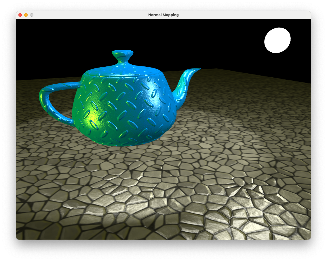
Fig. 9.14 Stone floor with no specular map applied.#
Move the camera around the floor and note how the mortar between the stones have specular highlights (an example of this can be seen in the bottom left-hand corner of Fig. 9.14). This isn’t very realistic as in real life mortar is rough and does not appear shiny. To overcome this we can apply a specular map to switch off the specular highlights for certain fragments.
To apply the specular map we added to the floor object we first need to add a specular map to the floor model. Where we added the diffuse and normal maps add a specular map using the following code
floor.addTexture("../objects/stones_specular.png", "specular");
We now need to make minor changes to the fragment shader. First, declare a sampler uniform for the specular map near to where we did the same for the diffuse and normal maps.
uniform sampler2D specularMap;
Then, whenever we calculate the specular lighting in the calculatePointLight(), calculateSpotlight() and calculateDirectionalLight() functions multiply by the colour of the textel from the specular map.
vec3 specular = ks * light.colour * pow(cosAlpha, Ns) * texture(specularMap, UV).rgb;
Compile and run the program and now you will notice that the mortar between the stones no longer have specular highlights.
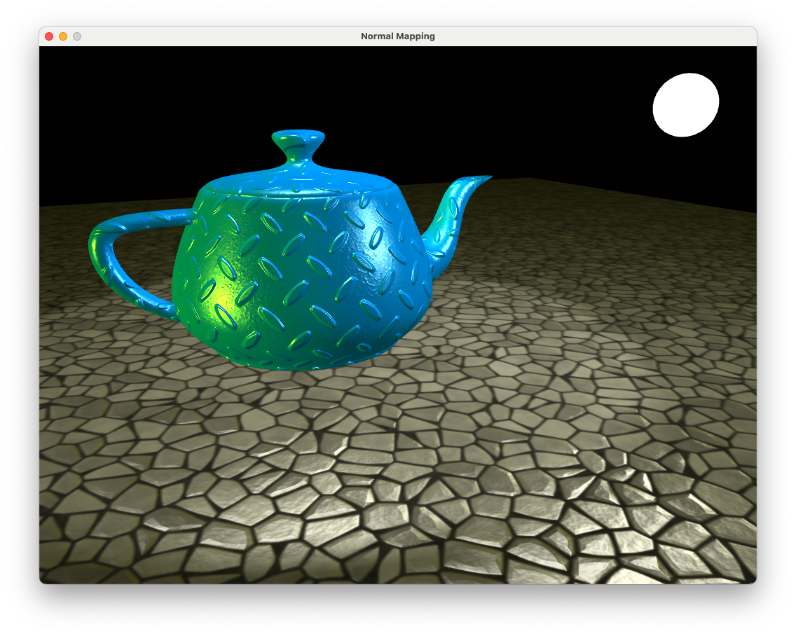
Fig. 9.15 Stone floor with specular map applied.#
9.4.1. Neutral maps#
We may not always want to apply a normal map or specular map to an object. Rather than writing a fragment shader for each case we can apply neutral maps which is a texture that when normal and specular mapping is applied it has no affect. Since the normal vector is calculated using
then if the normal maps has pixels with the RGB colour code (0.5, 0.5, 1) then all fragments will have a normal vector of (0, 0, 1) which is perpendicular to the surface.
A neutral specular map is simply a texture with all white pixels that have the RGB colour code (1, 1, 1) so multiplying this by the specular colour has no affect.
The neutral maps for normal and specular mapping are contained in the neutral_normal.png and neutral_specular.png files in the objects/ folder and are applied to a model when it is created. When we use the addTexture() Model class method the neutral maps are replaced.
9.5. Exercises#
Add another object using the .obj model
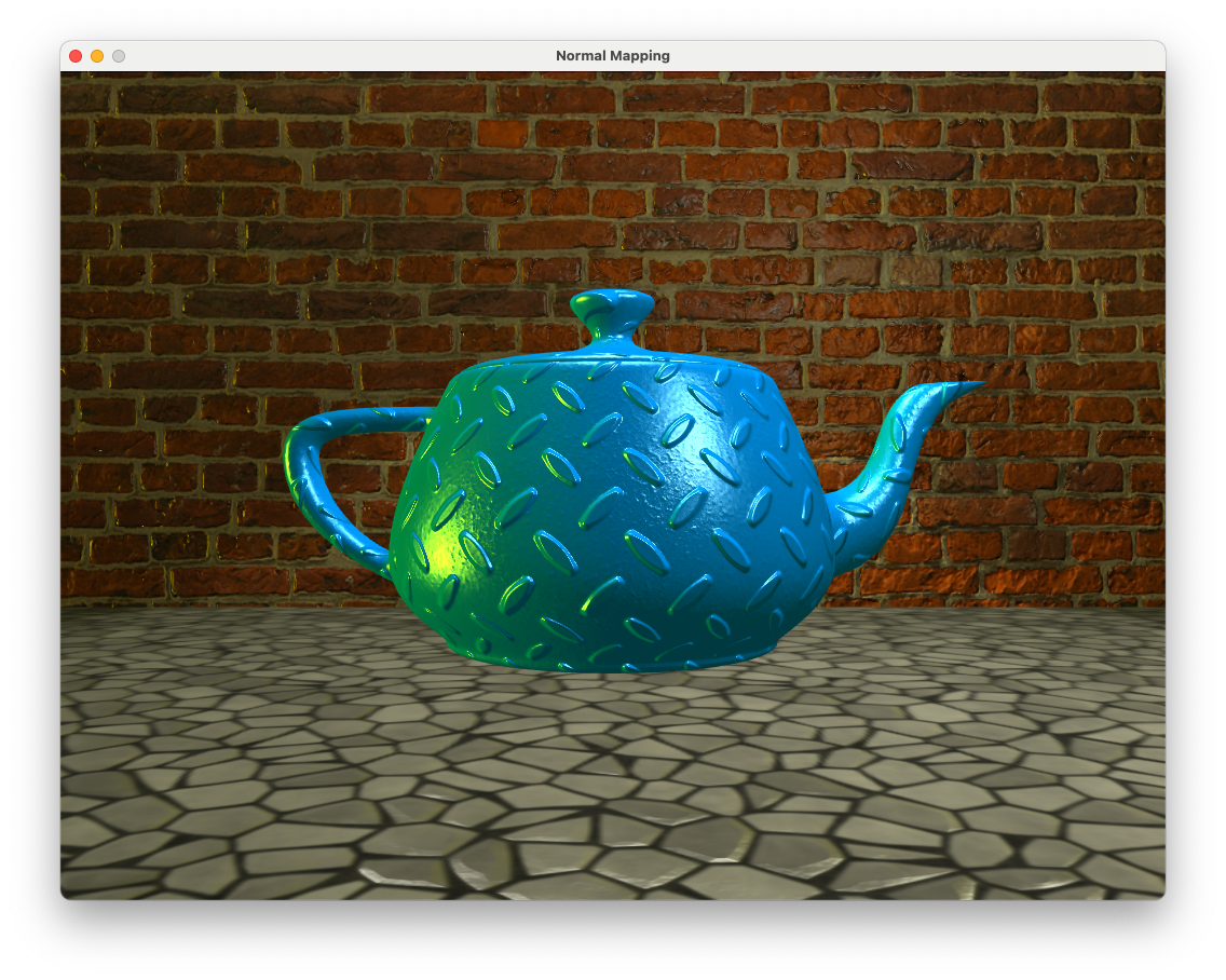
../objects/wall.objto your scene and position it at (0, 4, -2), scale it up by a factor of 5 in the x and z directions and rotate it 90\(^\circ\) about the x axis. Apply the diffuse map../objects/bricks_diffuse.png.
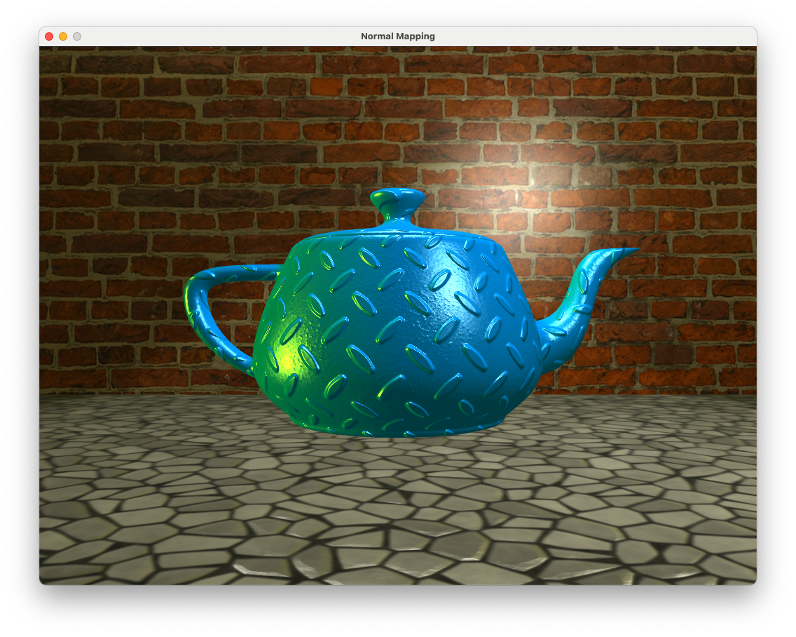
Apply the normal map
../objects/bricks_normal.pngto the wall object.
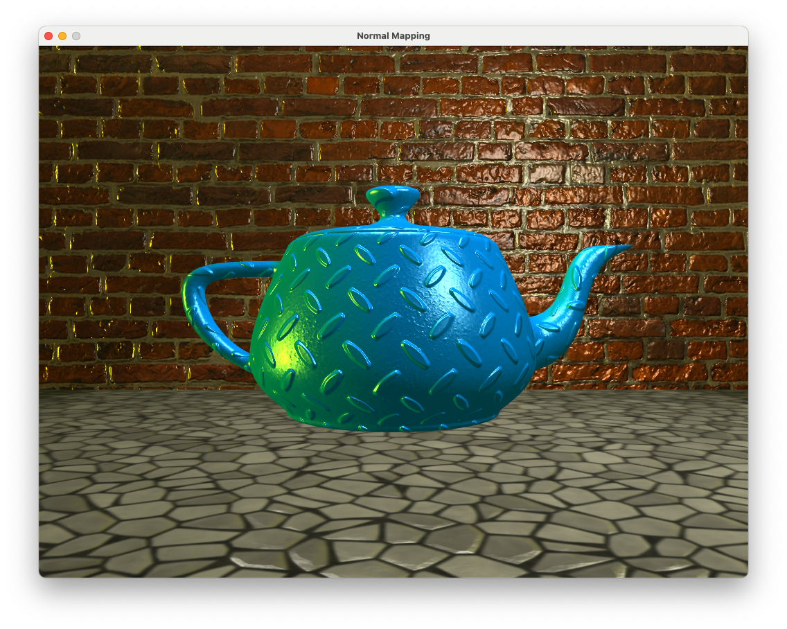
Apply the specular map
../objects/bricks_specular.pngto the wall object.