5. Transformations#
Computer graphics requires that shapes are manipulated in space by moving the shapes, shrinking or stretching, rotating and reflection to name a few. We call these manipulations transformations. We need a convenient way of telling the computer how to apply our transformations and for this we make use of matrices which we covered in the previous lab on vectors and matrices.
Each transformation has an associated transformation matrix which we use to multiply the vertex co-ordinates of a shape to calculate the vertex co-ordinates of the transformed shape. For example if \(A\) is a transformation matrix for a particular transformation and \((x,y,z)\) are the co-ordinates of a vertex then we apply the transformation using
where \((x',y',z')\) are the co-ordinates of the transformed point. Note that all vectors and co-ordinates are written as a column vector when multiplying by a matrix.
Note
The co-ordinate system used by OpenGL is a right-hand 3D co-ordinate system (on your right hand the thumb represents the \(x\)-axis, the index finger the \(y\)-axis and the middle finger the \(z\)-axis) with the \(x\)-axis pointing to the right, the \(y\)-axis point upwards and the \(z\)-axis pointing out of the screen towards the user (Fig. 5.1).

Fig. 5.1 The OpenGL co-ordinate system.#
5.1. Translation#
The translation transformation when applied to a set of points moves each point by the same amount. For example, consider the triangle in Fig. 5.2, each of the vertices has been translated by the same vector \(\mathbf{t}\) which has that effect of moving the triangle.

Fig. 5.2 Translation of a triangle by the translation vector \(\mathbf{t}= (t_x, t_y, t_z)\).#
A problem we have is that no transformation matrix exists for applying translation to the co-ordinates \((x, y, z)\), i.e., we can’t find a matrix \(Translate\) such that
We can use a trick where we use homogeneous co-ordinates. Homogeneous co-ordinates add another value, \(w\) say, to the \((x, y, z)\) co-ordinates (known as Cartesian co-ordinates) such that when the \(x\), \(y\) and \(z\) values are divided by \(w\) we get the Cartesian co-ordinates.
So if we choose \(w=1\) then we can write the Cartesian co-ordinates \((x, y, z)\) as the homogeneous co-ordinates \((x, y, z, 1)\) (remember that 4-element vector with the additional 1 in our vertex shader?). So how does that help us with our elusive translation matrix? Well we can now represent translation as a \(4 \times 4\) matrix
which is our desired translation. So the translation matrix for translating a set of points by the vector \(\mathbf{t} = (t_x, t_y, t_z)\) is
Important
Recall that OpenGL and glm use column-major order, so when coding transformation matrices into C++ we need to code the transpose of the matrix. So the translation matrix we are going to use is
5.1.1. Translation in OpenGL#
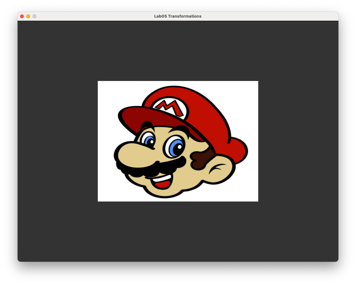
Now we know the mathematical theory behind applying a transformation lets apply it to OpenGL. Compile and run the Lab05_Transformations project and you should be presented with a rectangle textured with our old friend Mario as shown in Fig. 5.3.
Lets translate the rectangle \(0.4\) to the right and \(0.3\) upwards (remember we are dealing with normalised device co-ordinates so the window co-ordinates are between \(-1\) and \(1\)). The transposed transformation matrix to perform this translation is
In the Lab05_Transformations.cpp enter the following code just before we draw the triangles in the render loop.
// Define the translation matrix
glm::mat4 translate;
translate[3][0] = 0.4f, translate[3][1] = 0.3f, translate[3][2] = 0.0f;
We need a way of passing the translate matrix to the shader. We do this using a uniform like we did in the lab on texture maps. Add the following code after we have defined the translation matrix.
// Send the transformation matrix to the shader
glm::mat4 transformation = translate;
unsigned int transformationID;
transformationID = glGetUniformLocation(shaderID, "transformation");
glUniformMatrix4fv(transformationID, 1, GL_FALSE, &transformation[0][0]);
Here we have created another matrix called transformation and copied the translate matrix into it (we have done this because we will be combining different transformations into a single matrix later). Then after getting the location of the transformation uniform using the glGetUniformatLocation() function we send a reference to the first element of the transformation matrix to the shaders using glUniformMatrix4fv() function.
All we now have to do is modify the vertex shader to use the transformation matrix.
#version 330 core

// Inputs
layout(location = 0) in vec3 position;
layout(location = 1) in vec2 uv;

// Outputs
out vec2 UV;

// Uniforms
uniform mat4 transformation;

void main()
{
    // Output vertex position
    gl_Position = transformation * vec4(position, 1.0);

    // Output texture co-ordinates
    UV = uv;
}
The changes we have made here is to specify that we are passing the transformation matrix via a uniform and we multiply the homogeneous co-ordinates of the vertex position by this matrix. Compile and run the program and you should see that our rectangle has been translated to the right and up a bit as shown in Fig. 5.4.
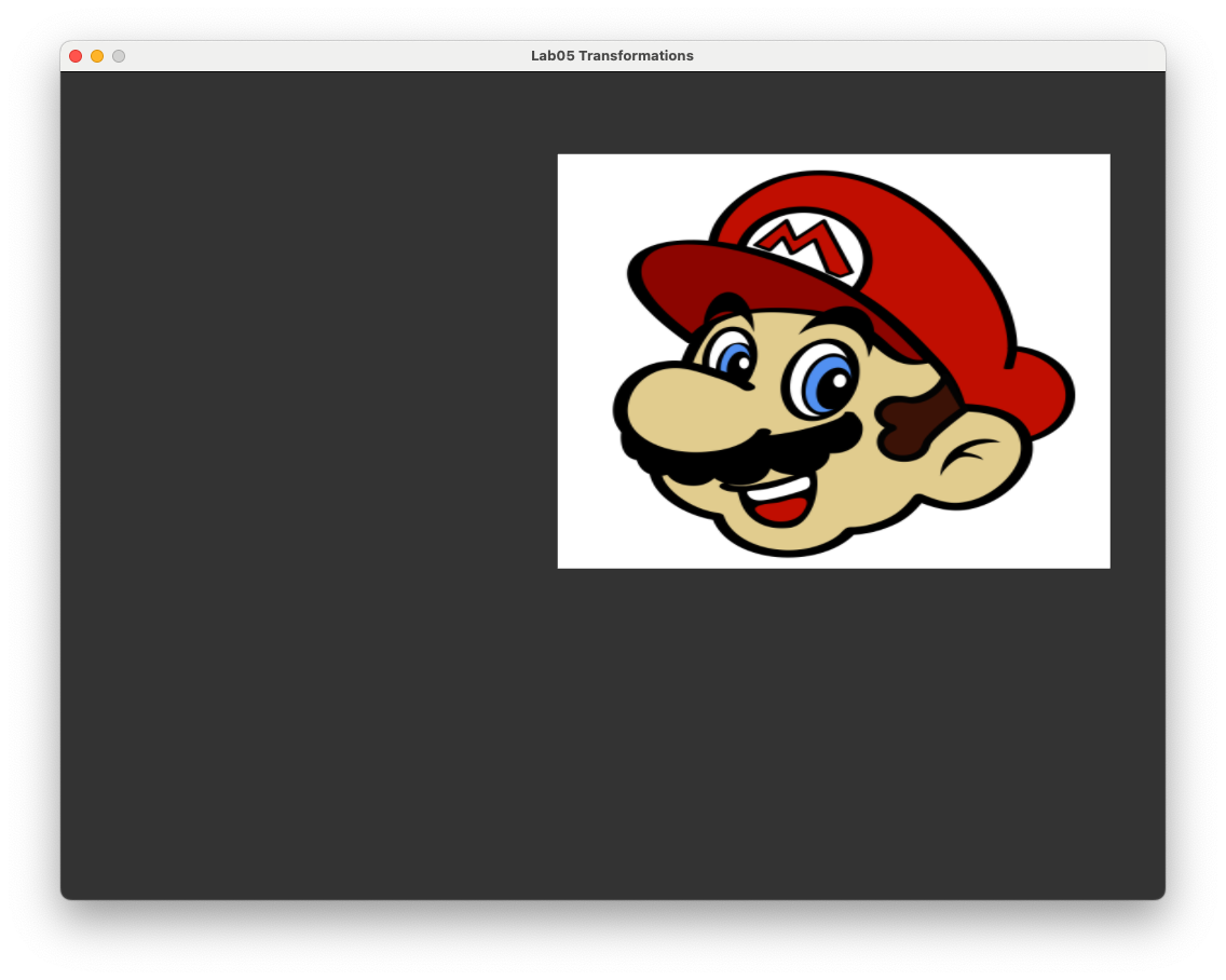
Fig. 5.4 A rectangle translated by the vector \((0.4, 0.3, 0)\).#
5.2. A Maths class#
Whilst it wasn’t particularly difficult to define the translation matrix, we may be doing this often so it makes sense to write a function to do this. Since we will also have other types of transformations we will create a Maths class to contain all of these function. If you open the maths.hpp file in the Lab05_Transformations project folder you will see that it is currently empty. Enter the following code to create a Maths class.
#pragma once

#include <iostream>
#include <cmath>
#include <glm/glm.hpp>
#include <glm/gtx/io.hpp>

// Maths class
class Maths
{
public:
    // Transformation matrices
    static glm::mat4 translate(const glm::vec3 &v);
};
Here we include the iostream, cmath and glm libraries before declaring our Maths class. We have also declared the method translate() that has a single input of a glm::vec3 object.
In the maths.cpp file enter the following method definition.
#include <common/maths.hpp>

glm::mat4 Maths::translate(const glm::vec3 &v)
{
    glm::mat4 translate(1.0f);
    translate[3][0] = v.x, translate[3][1] = v.y, translate[3][2] = v.z;
    return translate;
}
You will notice this is similar to the translate matrix we defined in the main program. We can now use this method to calculate any translation matrix. Comment out the code we used to define the translate matrix in the main program and enter the following.
glm::mat4 translate = Maths::translate(glm::vec3(0.4f, 0.3f, 0.0f));
Running the program you should see no change to the output but we can now easily define translation matrices. Experiment with different values for the translation vector to see the effects it has.
5.3. Scaling#
Scaling is one of the simplest transformation we can apply. Multiplying the \(x\), \(y\) and \(z\) co-ordinates of a point by a scalar quantity (a number) has the effect of moving the point closer or further away from the origin (0,0). For example, consider the triangle in Fig. 5.5. The \(x\), \(y\) and \(z\) co-ordinates of each vertex has been multiplied by \(s_x\), \(s_y\) and \(s_y\) respectively which has the effect of scaling the triangle and moving the vertices further away from the origin (in this case because \(s_x\), \(s_y\) and \(s_z\) are all greater than 1).

Fig. 5.5 Scaling a triangle centred at the origin.#
Since scaling is simply multiplying the co-ordinates by a number we have
so the scaling matrix for applying the scaling transformation is
Lets now apply scaling to our rectangle in OpenGL to increase its size by a factor of 0.4 in the horizontal direction and 0.3 in the vertical direction. The process is very similar to how we did the translation and since we have already created a uniform, passed it to the vertex shader and modified the vertex shader, all we need to do to apply shading is calculate the scaling matrix which is
Enter the following code into the main program after we defined the translation matrix.
// Define the scaling matrix
glm::mat4 scale;
scale[0][0] = 0.4f, scale[1][1] = 0.3f, scale[2][2] = 1.0f;
Note that the indices [0][0], [1][1] and [2][2] refer to the elements on the main diagonal of a glm::mat4 object. Also, set the transformation matrix equal to the scale matrix.
glm::mat4 transformation = scale;
Running the program you should see the image shown in Fig. 5.6.
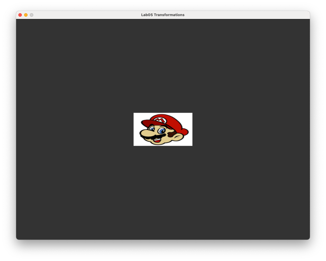
Fig. 5.6 A rectangle scaled by the vector \((0.4, 0.3, 1)\).#
Like with the translation matrix, it would be useful to have a Maths class method to calculate a scaling matrix. Add the following method prototype to the Maths class.
static glm::mat4 scale(const glm::vec3 &v);
Then define the method by entering the following code in the maths.cpp file.
glm::mat4 Maths::scale(const glm::vec3 &v)
{
    glm::mat4 scale(1.0f);
    scale[0][0]  = v.x; scale[1][1]  = v.y; scale[2][2] = v.z;
    return scale;
}
Check that the method works by commenting out the code used to define the scale matrix and add the following.
glm::mat4 scale = Maths::scale(glm::vec3(0.4f, 0.3f, 1.0f));
Running the program you should see no change to the image from Fig. 5.6.Experiment with different scaling vectors to see the affect this has.
Note
If scaling is applied to a shape that is not centred at \((0,0,0)\) then the transformed shape is distorted and its centre is moved from its original position (Fig. 5.7).

Fig. 5.7 Scaling applied to a triangle not centred at \((0,0,0)\).#
If the desired result is to resize the shape whilst keeping its dimensions and location the same we first need to translate the vertex co-ordinates by \(-\mathbf{c}\) where \(\mathbf{c}\) is the centre of volume for the shape so that it is at \((0,0,0)\). Then we can apply the scaling before translating by \(\mathbf{c}\) so that the centre of volume is back at the original position (Fig. 5.8).

Fig. 5.8 The steps required to scale a shape about its centre.#
5.4. Rotation#
As well as translating and scaling objects, the next most common transformation is the rotation of objects around the three co-ordinate axes \(x\), \(y\) and \(z\). We define the rotation anti-clockwise around each of the co-ordinate axes by an angle \(\theta\) when looking down the axes (Fig. 5.9).

Fig. 5.9 Rotation is assumed to be in the anti-clockwise direction when looking down the axis.#
The rotation matrices for achieving these rotations are
You don’t really need to know how these are derived but if you are curious you can click on the dropdown link below.
Derivation of the rotation matrices (click to show)
We will consider rotation about the \(z\)-axis and will restrict our co-ordinates to 2D.

Fig. 5.10 Rotating the vector \(\mathbf{a}\) anti-clockwise by angle \(\theta\) to the vector \(\mathbf{b}\).#
Consider Fig. 5.10 where the vector \(\mathbf{a}\) is rotated by angle \(\theta\) to the vector \(\mathbf{b}\). To get this rotation we first consider the rotation of the vector \(\mathbf{t}\), which has the same length as \(\mathbf{a}\) and points along the \(x\)-axis, by angle \(\phi\) to get to \(\mathbf{a}\). If we form a right-angled triangle (the blue one) then we know the length of the hypotenuse, \(|\mathbf{a}|\), and the angle so we can calculate the lengths of the adjacent and opposite sides using trigonometry. Remember our trig ratios (SOH-CAH-TOA)
so the length of the adjacent and opposite sides of the blue triangle is
Since \(a_x\) and \(a_y\) are the lengths of the adjacent and opposite sides respectively and \(|\mathbf{a}|\) is the length of the hypotenuse we have
Now consider the rotation from \(\mathbf{c}\) by the angle \(\phi + \theta\) to get to \(\mathbf{b}\). Using the same method as before we have
We can rewrite \(\cos(\phi+\theta)\) and \(\sin(\phi+\theta)\) using trigonometric identities
so
Since \( a_x = |\mathbf{a}| \cos(\phi)\) and \(a_y = |\mathbf{a}| \sin(\phi)\) then
which can be written using matrices as
so the transformation (non-transposed) matrix for rotating around the \(z\)-axis in 2D is
We need a \(4\times 4\) matrix to represent 3D rotation around the \(z\)-axis so we replace the 3rd and 4th row and columns with the 3rd and 4th row and column from the \(4\times 4\) identity matrix giving
The rotation matrices for the rotation around the \(x\) and \(y\) axes are derived using a similar process.
5.4.1. Rotation in OpenGL#
Lets rotate our original rectangle anti-clockwise about the \(z\)-axis by \(\theta = 45^\circ\). The transposed rotation matrix to do this is
Define the rotation matrix using the code below
// Define the rotation matrix
glm::mat4 rotate;
float angle = 45.0f * 3.1416f / 180.0f;
rotate[0][0] =  cos(angle), rotate[0][1] = sin(angle);
rotate[1][0] = -sin(angle), rotate[1][1] = cos(angle);
Here we also needed to convert \(45^\circ\) into radians since OpenGL expects angles to be in radians (1 radian is equal to \(\pi/180\) degrees). Set the transformation matrix equal to the rotate matrix, run the program and you should see the rotated rectangle shown in Fig. 5.11.
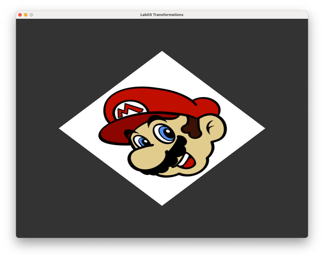
Fig. 5.11 Rectangle rotated anti-clockwise about the \(z\)-axis by \(45^\circ\).#
5.4.2. Axis-angle rotation#
The three rotation transformations are only useful if we want to only rotate around one of the three co-ordinate axes. A more useful transformation is the rotation around the axis that points in the direction of a vector, \(\mathbf{v}\) say, which has its tail at (0,0,0) (Fig. 5.12).

Fig. 5.12 Axis-angle rotation.#
The transposed transformation matrix for rotation around a unit vector \(\hat{\mathbf{v}} = (v_x, v_y, v_z)\), anti-clockwise by angle \(\theta\) when looking down the vector is.
Again, you don’t really need to know how this is derived but if you are curious click on the dropdown link below.
Derivation of the axis-angle rotation matrix (click to show)
The rotation about the unit vector \(\hat{\mathbf{v}} = (v_x, v_y, v_z)\) by angle \(\theta\) is the composition of 5 separate rotations:
Rotate \(\hat{\mathbf{v}}\) around the \(x\)-axis so that it is in the \(xz\)-plane (the \(y\) component of the vector is 0);
Rotate the vector around the \(y\)-axis so that it points along the \(z\)-axis (the \(x\) and \(y\) components are 0 and the \(z\) component is a positive number);
Perform the rotation around the \(z\)-axis;
Reverse the rotation around the \(y\)-axis;
Reverse the rotation around the \(x\)-axis.
The rotation around the \(x\)-axis is achieved by forming a right-angled triangle in the \(yz\)-plane where the the angle of rotation \(\theta\) has an adjacent side of length \(v_z\), an opposite side of length \(v_y\) and a hypotenuse of length \(\sqrt{v_y^2 + v_z^2}\) (Fig. 5.13).

Fig. 5.13 Rotate \(\mathbf{v}\) around the \(x\)-axis#
Therefore \(\cos(\theta) = \dfrac{v_z}{\sqrt{v_y^2 + v_z^2}}\) and \(\sin(\theta) = \dfrac{v_y}{\sqrt{v_y^2 + v_z^2}}\) so the rotation matrix is
The rotation around the \(y\)-axis is achieved by forming another right-angled triangle in the \(xz\)-plane where \(\theta\) has an adjacent side of length \(\sqrt{v_y^2 + v_z^2}\), an opposite side of length \(v_x\) and a hypotenuse of length 1 since \(\hat{\mathbf{v}}\) is a unit vector (Fig. 5.14).

Fig. 5.14 Rotate around the \(y\)-axis#
Therefore \(\cos(\theta) = \sqrt{v_y^2 + v_z^2}\) and \(\sin(\theta) = v_x\). Note that here we are rotating in the clockwise direction so the rotation matrix is
Now that the vector points along the \(z\)-axis we perform the rotation so the rotation matrix for this is
The reverse rotation around the \(y\) and \(x\) axes is simply the rotation matrices \(R_2\) and \(R_1\) with the negative sign for \(\sin(\theta)\) swapped
Multiplying all of the separate matrices together gives
Substituting \(v_y^2 + v_z^2 = 1 - v_x^2\) and the matrix simplifies to
5.4.3. Axis-angle rotation in OpenGL#
The rotations around the three co-ordinates axis can be calculated using the axis-angle rotation matrix (by letting \(\hat{\mathbf{v}}\) be \((1,0,0)\), \((0,1,0)\) or \((0,0,1)\) for rotating around the \(x\), \(y\) and \(z\) axes respectively) so it makes sense to define a single function for rotation using (5.3). Define a couple of functions in the Maths class by entering the following code.
static float radians(float angle);
static glm::mat4 rotate(const float &angle, glm::vec3 v);
Then define these methods by entering the following code in the maths.cpp file.
float Maths::radians(float angle)
{
    return angle * 3.1416f / 180.0f;
}

glm::mat4 Maths::rotate(const float &angle, glm::vec3 v)
{
    v = glm::normalize(v);
    float c = cos(angle);
    float s = sin(angle);
    float x2 = v.x * v.x, y2 = v.y * v.y, z2 = v.z * v.z;
    float xy = v.x * v.y, xz = v.x * v.z, yz = v.y * v.z;
    float xs = v.x * s,   ys = v.y * s,   zs = v.z * s;

    glm::mat4 rotate;
    rotate[0][0] = (1 - c) * x2 + c;
    rotate[0][1] = (1 - c) * xy + zs;
    rotate[0][2] = (1 - c) * xz - ys;
    rotate[1][0] = (1 - c) * xy - zs;
    rotate[1][1] = (1 - c) * y2 + c;
    rotate[1][2] = (1 - c) * yz + xs;
    rotate[2][0] = (1 - c) * xz + ys;
    rotate[2][1] = (1 - c) * yz - xs;
    rotate[2][2] = (1 - c) * z2 + c;

    return rotate;
}
Check that the rotate() method works by commenting out the code used to define the rotation matrix and add the following.
float angle      = Maths::radians(45.0f);
glm::mat4 rotate = Maths::rotate(angle, glm::vec3(0.0f, 0.0f, 1.0f));
Running the program you should see no change to the image shown in Fig. 5.11. Experiment with different angles and rotation vectors to see the affects this has.
5.5. Composite transformations#
So far we have performed translation, scaling and rotation transformations on our rectangle separately. What if we wanted to combine these transformations so that we can control the size, rotation and position of the rectangle? If we apply the transformations in the order scale \(\rightarrow\) rotate \(\rightarrow\) translate then applying the scaling we have
Next applying rotation to the scaled co-ordinates we have
Finally applying translation to the scaled and rotated co-ordinates we have
\(Translate \cdot Rotate \cdot Scale\) is a single \(4 \times 4\) transformation matrix that combines the three transformations known as the composite transformation matrix. Note the order that the translations are applied to the co-ordinates is read from right to left so here we have scale \(\to\) rotate \(\to\) translate.
5.5.1. Composite transformations in OpenGL#
Lets apply scaling, rotation and translation (in that order) to our rectangle. Since we have already calculated the separate transformation matrices all we need to do is to multiply them together and set it equal to transformation.
glm::mat4 transformation = translate * rotate * scale;
After compiling and running the program you should see the image shown in Fig. 5.15.
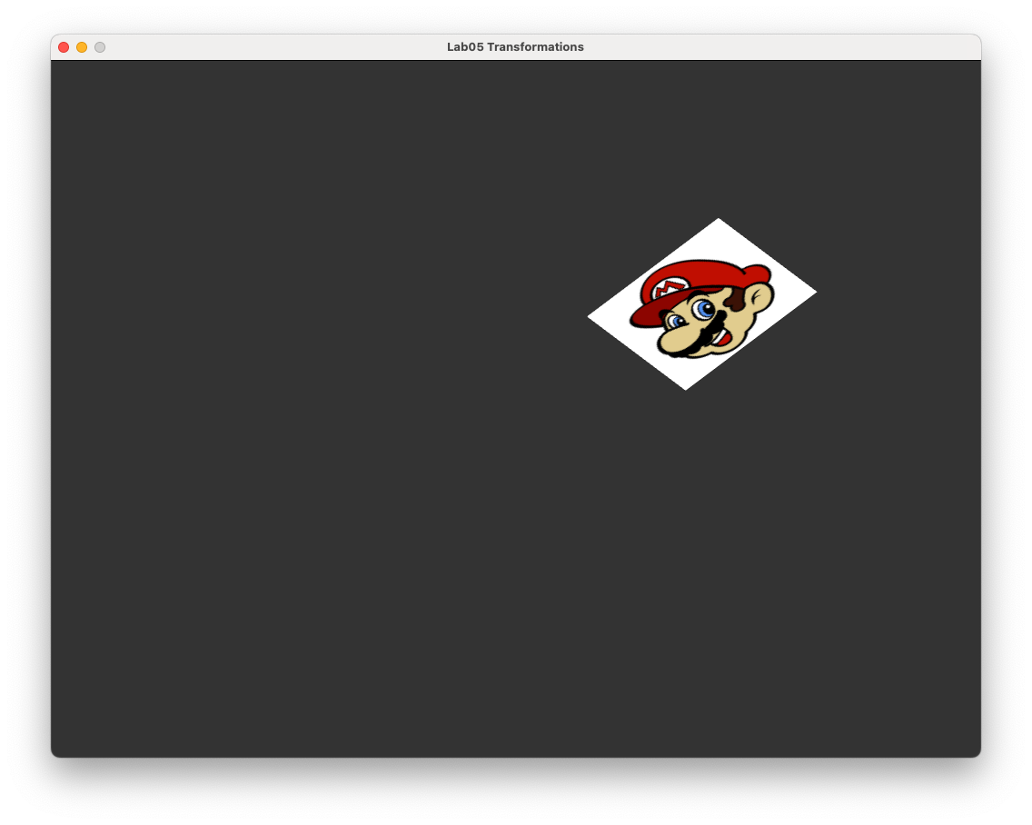
Fig. 5.15 Scaling, rotation and translation applied to the textured rectangle.#
5.6. Animating the rectangle#
It may appear that our application is displaying a static image of the textured rectangle but what is actually happening is that the window is constantly being updated with new frame buffers as and when they have been calculated. We can animate our rectangle by applying the transformations within the render loop.
We are going to animate our rectangle so that is rotates around its own centre. To do this we are going to use the time the has elapsed since the application was started to calculate the rotation angle. Enter the following code just before the transformation matrix is sent to the shader
// Animate rectangle
float angle         = Maths::radians(glfwGetTime() * 360.0f / 3.0f);
glm::mat4 translate = Maths::translate(glm::vec3(0.4f, 0.3f, 0.0f));
glm::mat4 scale     = Maths::scale(glm::vec3(0.4f, 0.3f, 0.0f));
glm::mat4 rotate    = Maths::rotate(angle, glm::vec3(0.0f, 0.0f, 1.0f));
Here we use the glfwGetTime() function to get the time of the current frame since the application was started and use it to calculate the rotation angle so that the rectangle performs one complete rotation every 3 seconds. Compile and run the program and you should see something similar to the following.
When calculating the composite transformation matrix the order in which we multiply the individual transformations will determine the effects of the composite transformation. To see this lets translate the rectangle first before rotating it by changing the transformation calculation to the following.
glm::mat4 transformation = rotate * translate * scale;
Compile and run the program and we have something quite different.
What has happened here is the rectangle has been scaled and translated so that its centre is now at \((0.4, 0.3, 0)\). Then when rotation is applied the triangle is rotated about the origin.
5.7. Exercises#
Scale the original rectangle so that it is a quarter of the original size and apply translation so that the rectangle moves anti-clockwise around a circle centred at the window centre with radius 0.5 and completes one full rotation every 5 seconds. Hint: the co-ordinates of points on a circle centered at \((0,0)\) with radius \(r\) can be calculated using \(x = r\cos(t)\) and \(y = r\sin(t)\) where \(t\) is some number.
Rotate your rectangle from exercise 1 in a clockwise rotation about its centre at twice the rotation speed used in exercise 1.
Scale your rectangle from exercise 2 so that it grows and shrinks about its centre. Hint: The \(\sin(t)\) function oscillates between 0 and 1 as \(t\) increases.
Create a simple screensaver by doing the following:
Before the
main()function, define two 3-element vectors for the position and velocity with initial values \(\mathbf{p} = (0,0,0)\) and \(\mathbf{v} = (0.01, 0.005, 0)\) respectivelyInside the render loop, calculate the new centre position using \(\mathbf{p} = \mathbf{p} + \mathbf{v}\)
Scale the original rectangle so that it is one fifth its original size and translate the rectangle so that its center is at \(\mathbf{p}\)
Reflect the rectangle off the edges of the window by reversing the sign of the elements of the velocity vector when the center of the rectangle gets to within 0.1 of the window edge.
Run your program from exercise 4 until the rectangle perfectly hits a corner (just kidding).