6. 3D Worlds

In the previous lab we looked at the transformations can can be applied to the vertex co-ordinates \((x, y, z, 1)\) but all of our examples were using transformations in 2D. In this lab we will take the step into the third spatial dimension and look at 3D worlds.

6.1. 3D models

To demonstrate building a simple 3D world we are going to need a 3D object. One of the simplest 3D objects is a unit cube which is a cube centred at (0,0,0) and has side lengths of 2 parallel to the co-ordinate axes (Fig. 6.1) so the co-ordinates of the 8 corners of the cube are combinations of \(-1\) and \(1\). Since we use triangles as our base shape a cube consists of 12 triangles (6 sides each made out of 2 triangles).

Fig. 6.1 A unit cube centred at \((0,0,0)\) with side lengths of 2.

Open the Lab06_3D_Worlds.cpp file in the Lab06_3D_Worlds project and you will see that the vertices, uv and indices arrays have been defined for our unit cube.

// Define cube object
// Define vertices
const float vertices[] = {
    // front
    -1.0f, -1.0f,  1.0f,    //              + ------ +
     1.0f, -1.0f,  1.0f,    //             /|       /|
     1.0f,  1.0f,  1.0f,    //   y        / |      / |
    -1.0f, -1.0f,  1.0f,    //   |       + ------ +  |
     1.0f,  1.0f,  1.0f,    //   + - x   |  + ----|- +
    -1.0f,  1.0f,  1.0f,    //  /        | /      | /
    // right                // z         |/       |/
     1.0f, -1.0f,  1.0f,    //           + ------ +
     1.0f, -1.0f, -1.0f,
     1.0f,  1.0f, -1.0f,
     1.0f, -1.0f,  1.0f,
     1.0f,  1.0f, -1.0f,
     1.0f,  1.0f,  1.0f,
    // etc.
};

// Define texture coordinates
const float uv[] = {
    // front
    0.0f, 0.0f,     // vertex co-ordinates are the same for each side
    1.0f, 0.0f,     // of the cube so repeat every six vertices
    1.0f, 1.0f,
    0.0f, 0.0f,
    1.0f, 1.0f,
    0.0f, 1.0f,
    // right
    0.0f, 0.0f,
    1.0f, 0.0f,
    1.0f, 1.0f,
    0.0f, 0.0f,
    1.0f, 1.0f,
    0.0f, 1.0f,
    // etc.
};

// Define indices
unsigned int indices[] = {
    0,   1,  2,  3,  4,  5,     // front
    6,   7,  8,  9, 10, 11,     // right
    12, 13, 14, 15, 16, 17,     // back
    18, 19, 20, 21, 22, 23,     // left
    24, 25, 26, 27, 28, 29,     // bottom
    30, 31, 32, 33, 34, 35      // top
};

If you compile and run this program you will see that the crate texture fills the window.

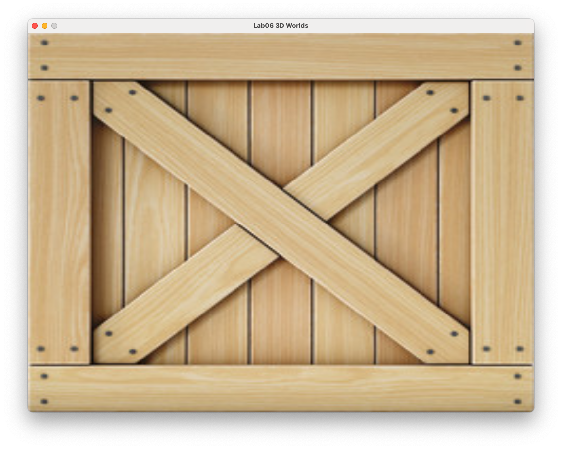
Fig. 6.2 A unit cube.

---

6.2. Co-ordinate systems

OpenGL uses a co-ordinate system with the \(x\) axis pointing horizontally to the right, the \(y\) axis pointing vertically upwards and the \(z\) axis pointing horizontally towards the viewer. To simplify things when it comes to displaying the 3D world, the axes are limited to a range from \(-1\) to \(1\) so any object outside of this range will not be shown on the display. These are known as Normalised Device Co-ordinates (NDC).

Fig. 6.3 Normalised Device Co-ordinates (NDC)

The steps used in the creation of a 3D world and eventually displaying it on screen requires that we transform through several intermediate co-ordinate systems:

• Model space – each individual 3D object that will appear in the 3D world is defined in its own space usually with the volume centre of the object at \((0,0,0)\) to make the transformations easier

• World space – the 3D world is constructed by transforming the individual 3D objects using translation, rotation and scaling transformations

• View space – the world space is transformed so that it is viewed from \((0,0,0)\) looking down the \(z\)-axis

• Screen space – the view space is transformed so that the co-ordinates are expressed using normalised device co-ordinates

Fig. 6.4 Transformations between the model, world, view and screen spaces.

6.3. Model, view and projection matrices

We saw in 5. Transformations that we apply a transformation by multiplying the object co-ordinates by a transformation matrix. Since we are transforming between difference co-ordinate spaces we have 3 main transformation matrices

• Model matrix - transforms the model space co-ordinates for the objects to the world space

• View matrix - transforms the world space co-ordinates to the view space co-ordinates

• Projection matrix - transforms the view space co-ordinates to the screen space NDC co-ordinates

6.3.1. The Model matrix

In 5. Transformations we saw that we can combine transformations such as translation, scaling and rotation by multiplying the individual transformation matrices together. Lets compute a model matrix for our cube where it is scaled down by a factor of 0.5 in each co-ordinate direction, rotated about the \(y\)-axis using the time of the current frame as the rotation angle and translated backwards down the \(z\)-axis so that its centre is at \((0, 0, -2)\). Add the following code inside the rendering loop before we call the glDrawElements() function.

// Calculate the model matrix
float angle         = Maths::radians(glfwGetTime() * 360.0f / 3.0f);
glm::mat4 translate = Maths::translate(glm::vec3(0.0f, 0.0f, -2.0f));
glm::mat4 scale     = Maths::scale(glm::vec3(0.5f, 0.5f, 0.5f));
glm::mat4 rotate    = Maths::rotate(angle, glm::vec3(0.0f, 1.0f, 0.0f));
glm::mat4 model     = translate * rotate * scale;

Here we have calculated the individual transformation matrices for translation, scaling and rotation and multiply them together to create the model matrix. The rotation angle has been calculated using the time of the current frame so that the cube will perform one full rotation every 3 seconds.

6.3.2. The View matrix

To view the world space we create a virtual camera and place it in the world space. We need to translate the whole of the world space so that the camera is at \((0,0,0)\) and the rotate the world space so that the camera is pointing down the \(z\)-axis (Fig. 6.5).

Fig. 6.5 The view space.

To calculate the world space to view space transformation we require three vectors

• \(\mathbf{eye}\) – the co-ordinates of the camera position

• \(\mathbf{target}\) – the co-ordinates of the target point that the camera is pointing

• \(\mathbf{worldUp}\) – a vector pointing straight up in the world space which allows us to orientate the camera, this is usually \((0, 1, 0)\)

Fig. 6.6 The vectors used in the transformation to the view space.

The \(\mathbf{eye}\) and \(\mathbf{target}\) vectors are either determined by the user through keyboard, mouse or controller inputs or through some predetermined routine. To determine the view space transformation we first translate the camera position by the vector \(-\mathbf{eye}\) so that it is at \((0, 0, 0)\) using the following translation matrix

\[\begin{split} \begin{align*} Translate = \begin{pmatrix} 1 & 0 & 0 & -\mathbf{eye}_x \\ 0 & 1 & 0 & -\mathbf{eye}_y \\ 0 & 0 & 1 & -\mathbf{eye}_z \\ 0 & 0 & 0 & 1 \end{pmatrix} \end{align*}, \end{split}\]

The next step is to align the world space so that the direction vector is pointing down the \(z\)-axis. To do this we use vectors \(\mathbf{right}\), \(\mathbf{up}\) and \(\mathbf{front}\) which are unit vectors at right-angles to each other the point in directions relative to the camera (Fig. 6.6).

The \(\mathbf{front}\) vector points directly forward of the camera and is calculated using

\[ \mathbf{front} = \frac{\mathbf{target} - \mathbf{eye}}{\| \mathbf{target} - \mathbf{eye}\|}.\]

The \(\mathbf{right}\) vector points to the right of the camera so is at right-angles to both the \(\mathbf{front}\) and \(\mathbf{worldUp}\) vectors. We can use the cross product between the two vectors to calculate this (note that the order of the vectors is important).

\[ \mathbf{right} = \frac{\mathbf{front} \times \mathbf{worldUp}}{\| \mathbf{front} \times \mathbf{worldUp} \|}.\]

The \(\mathbf{up}\) vector points in the up direction of the camera and is at right-angles to the \(\mathbf{front}\) and \(\mathbf{right}\) vectors we have already calculated. So this can be calculated using another cross product (we don’t need to normalise this this both \(\mathbf{right}\) and \(\mathbf{front}\) are unit vectors).

\[ \mathbf{up} = \mathbf{right} \times \mathbf{front}.\]

Once these vectors have been calculated the transformation matrix to rotate the \(\mathbf{front}\) vector so that it points down the \(z\)-axis is

\[\begin{split} Rotate = \begin{pmatrix} \mathbf{right}_x & \mathbf{right}_y & \mathbf{right}_z & 0 \\ \mathbf{up}_x & \mathbf{up}_y & \mathbf{up}_z & 0 \\ -\mathbf{front}_x & -\mathbf{front}_y & -\mathbf{front}_z & 0 \\ 0 & 0 & 0 & 1 \end{pmatrix}.\end{split}\]

The translation matrix and rotation matrix are multiplied together to form the view matrix which transforms the world space co-ordinates to the view space.

\[\begin{split} \begin{align*} \view &= Rotate \cdot Translate \\ &= \begin{pmatrix} \mathbf{right}_x & \mathbf{right}_y & \mathbf{right}_z & 0 \\ \mathbf{up}_x & \mathbf{up}_y & \mathbf{up}_z & 0 \\ -\mathbf{front}_x & -\mathbf{front}_y & -\mathbf{front}_z & 0 \\ 0 & 0 & 0 & 1 \end{pmatrix} \begin{pmatrix} 1 & 0 & 0 & -\mathbf{eye}_x \\ 0 & 1 & 0 & -\mathbf{eye}_y \\ 0 & 0 & 1 & -\mathbf{eye}_z \\ 0 & 0 & 0 & 1 \end{pmatrix} \\ &= \begin{pmatrix} \mathbf{right}_x & \mathbf{right}_y & \mathbf{right}_z & -\mathbf{eye}_x \cdot \mathbf{right} \\ \mathbf{up}_x & \mathbf{up}_y & \mathbf{up}_z & -\mathbf{eye}_y \cdot \mathbf{up} \\ -\mathbf{front}_x & -\mathbf{front}_y & -\mathbf{front}_z & \mathbf{eye}_z \cdot \mathbf{front} \\ 0 & 0 & 0 & 1 \end{pmatrix} \end{align*} \end{split}\]

So the transposed view matrix is

(6.1)\[\begin{split} \view = \begin{pmatrix} \mathbf{right}_x & \mathbf{up}_x & -\mathbf{front}_x & 0 \\ \mathbf{right}_y & \mathbf{up}_y & -\mathbf{front}_y & 0 \\ \mathbf{right}_z & \mathbf{up}_z & -\mathbf{front}_z & 0 \\ -\mathbf{eye} \cdot \mathbf{right} & -\mathbf{eye} \cdot \mathbf{up} & \mathbf{eye} \cdot \mathbf{front} & 1 \\ \end{pmatrix} \end{split}\]

Lets move the camera to the right, back and up a bit so that it is at \((1, 1, 1)\) looking towards the center of the cube which is at \((0, 0, -2)\). Add the following code after we have calculated the model matrix.

// Calculate the view matrix
glm::vec3 eye     = glm::vec3(1.0f, 1.0f, 1.0f);
glm::vec3 target  = glm::vec3(0.0f, 0.0f, -2.0f);
glm::vec3 worldUp = glm::vec3(0.0f, 1.0f, 0.0f);
glm::vec3 front   = glm::normalize(target - eye);
glm::vec3 right   = glm::normalize(glm::cross(front, worldUp));
glm::vec3 up      = glm::cross(right, front);

glm::mat4 view;
view[0][0] = right.x, view[0][1] = up.x, view[0][2] = -front.x;
view[1][0] = right.y, view[1][1] = up.y, view[1][2] = -front.y;
view[2][0] = right.z, view[2][1] = up.z, view[2][2] = -front.z;
view[3][0] = -glm::dot(eye, right);
view[3][1] = -glm::dot(eye, up);
view[3][2] =  glm::dot(eye, front);

Here we have specified the \(\mathbf{eye}\), \(\mathbf{target}\) and \(\mathbf{worldUp}\) vectors and use them to calculate the \(\mathbf{front}\), \(\mathbf{right}\) and \(\mathbf{up}\) camera vectors. We then use these to calculate the view matrix.

6.3.3. The Projection matrix

The next step is to project the view space onto the screen space. The simplest type of projection is orthographic projection where the co-ordinates in the view space are transformed to the screen space by simple translation and scaling transformations.

The region of the view space that will form the screen space is defined by a cuboid bounded by a left, right, bottom, top, near and far clipping planes. Any objects outside of the cuboid are clipped (Fig. 6.7).

Fig. 6.7 Orthographic projection.

The transpose of the orthographic projection matrix is calculated using

\[\begin{split} \begin{align*} Projection_{orth} = \begin{pmatrix} \dfrac{2}{right - left} & 0 & 0 & 0 \\ 0 & \dfrac{2}{top - bottom} & 0 & 0 \\ 0 & 0 & \dfrac{2}{near - far} & 0 \\ -\dfrac{right + left}{right - left} & -\dfrac{top + bottom}{top - bottom} & \dfrac{near + far}{near - far} & 1 \end{pmatrix} \end{align*}, \end{split}\]

where \(left\), \(right\), \(bottom\), \(top\), \(near\) and \(far\) are the co-ordinates of the edges of the visible space. You don’t really need to know how this matrix is derived but if you are interested click on the dropdown link below.

Derivation of the orthographic projection matrix

To derive the orthographic projection we first need to translate the co-ordinates so that the centre of the cuboid that represents the clipping volume to \((0,0,0)\). The centre co-ordinates are calculated using the average of the edge co-ordinates, e.g., for the \(x\) co-ordinate this would be \(\dfrac{right + left}{2}\), so the translation matrix is

\[\begin{split} \begin{align*} Translate = \begin{pmatrix} 1 & 0 & 0 & -\dfrac{right + left}{2} \\ 0 & 1 & 0 & -\dfrac{top + bottom}{2} \\ 0 & 0 & 1 & \dfrac{near + far}{2} \\ 0 & 0 & 0 & 1 \end{pmatrix} \end{align*} \end{split}\]

The second step is to scale the clipping volume so that the co-ordinates are between \(-1\) and \(1\). This is done by dividing the distance between the edges of the screen space by the distance between the clipping planes, e.g., for the \(x\) co-ordinate this would be \(\dfrac{1 - (-1)}{right - left}=\dfrac{2}{right - left}\), so the scaling matrix is

\[\begin{split} \begin{align*} Scale = \begin{pmatrix} \dfrac{2}{right - left} & 0 & 0 & 0 \\ 0 & \dfrac{2}{top - bottom} & 0 & 0 \\ 0 & 0 & \dfrac{2}{near - far} & 0 \\ 0 & 0 & 0 & 1 \end{pmatrix}. \end{align*} \end{split}\]

Combining the translation and scaling matrices gives the orthographic projection matrix

\[\begin{split} \begin{align*} Projection_{orth} &= Translate \cdot Scale \\ &= \begin{pmatrix} \dfrac{2}{right - left} & 0 & 0 & -\dfrac{right + left}{right - left} \\ 0 & \dfrac{2}{top - bottom} & 0 & -\dfrac{top + bottom}{top - bottom} \\ 0 & 0 & \dfrac{2}{near - far} & \dfrac{near + far}{near - far} \\ 0 & 0 & 0 & 1 \end{pmatrix} \end{align*} \end{split}\]

Lets calculate the orthographic projection matrix using \(left = -2\), \(right = 2\), \(bottom = -2\), \(top = 2\), \(near = 0\), \(far = 10\). Add the following code after we have calculated the view matrix.

// Calculate orthographic projection matrix
float left   = -2.0f, right_ = 2.0f;
float bottom = -2.0f, top    = 2.0f;
float near   =  0.0f, far    = 10.0f;

glm::mat4 projection;
projection[0][0] = 2.0f / (right_ - left);
projection[1][1] = 2.0f / (top - bottom);
projection[2][2] = 2.0f / (near - far);
projection[3][0] = -(right_ + left) / (right_ - left);
projection[3][1] = -(top + bottom) / (top - bottom);
projection[3][2] =  (near + far) / (near - far);

6.3.4. The MVP matrix

Now that we have the model, view and projection matrices we need to apply them to our objects. We could do this in our main() function but this would mean sending lots of vertex buffers to the GPU and very inefficient. Much better to send a single \(4 \times 4\) matrix to the shader and perform the calculations using the GPU since the vertex buffer is already in the GPU memory.

So in our main() function we combine the model, view and projection matrices to form a single matrix called the \(MV\!P\) matrix.

\[ MV\!P = Projection \cdot \view \cdot \model. \]

We need a way to send the \(MV\!P\) matrix to the vertex shader. We do this using a uniform in the same way as we did for the texture locations in 3. Textures, enter the following code after we have calculated the projection matrix.

// Send MVP matrix to the vertex shader
glm::mat4 MVP = projection * view * model;
glUniformMatrix4fv(glGetUniformLocation(shaderID, "MVP"), 1, GL_FALSE, &MVP[0][0]);

Here after calculating the \(MV\!P\) matrix we get the location of the uniform and point OpenGL to the first element of the matrix using the glUniformMatrix4fv() function.

We also need to update the vertex shader so that is uses the \(MV\!P\) matrix. Edit the vertexShader.glsl file in the Lab06_3D_Worlds project so that the gl_Position vector is calculated by applying the \(MV\!P\) matrix to the vertex position.

#version 330 core

// Inputs
layout(location = 0) in vec3 position;
layout(location = 1) in vec2 uv;

// Outputs
out vec2 UV;

// Uniforms
uniform mat4 mvp;

void main()
{
    // Output vertex position
    gl_Position = mvp * vec4(position, 1.0);
    
    // Output texture co-ordinates
    UV = uv;
}

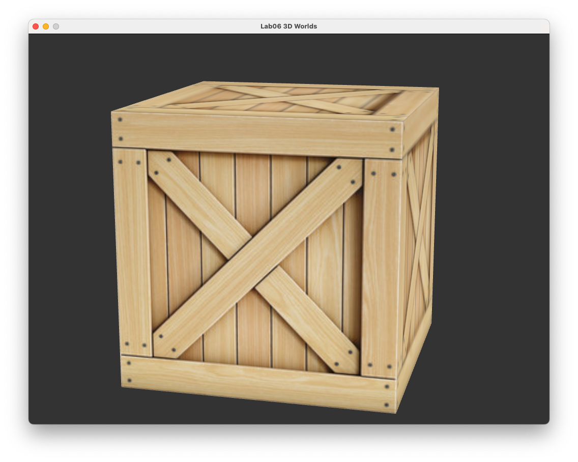
Compile and run the program and you should see the following.

---

6.4. The depth test

Our rendering of the cube doesn’t look quite right. What is happening here is that some parts of the sides of the cube that are further away from where we are viewing it (e.g., the bottom side) have been rendered after the sides that are closer to us (Fig. 6.8).

Fig. 6.8 Rendering the far triangle after the near triangle.

To overcome this issue OpenGL uses a depth test when computing the fragment shader. When OpenGL creates a frame buffer it also creates another buffer called a z buffer (or depth buffer) where the \(z\) co-ordinate of each pixel in the frame buffer is stored and initialises all the values to \(-1\) (the furthest possible \(z\) co-ordinate in the screen space). When the fragment shader is called it checks whether the fragment has a \(z\) co-ordinate more than that already stored in the depth buffer and if so it updates the colour of the fragment and stores its \(z\) co-ordinate in the depth-buffer as the current nearest fragment (if the fragment has a \(z\) co-ordinate less than what is already in the depth buffer the fragment shader does nothing). This means once the fragment shader has been called for all fragments of all objects, the pixels contain colours of the objects closest to the camera.

To enable depth testing we simply add the following function before after the creation of the window.

// Enable depth test
glEnable(GL_DEPTH_TEST);

We also need to clear the depth buffer at the start of each frame, change glClear(GL_COLOR_BUFFER_BIT); to the following.

// Clear the window
glClear(GL_COLOR_BUFFER_BIT | GL_DEPTH_BUFFER_BIT);

Make these changes to your code and you should get a much better result.

---

6.5. Perspective projection

The problem with using orthographic projection is that is does not give us any clues to how far an object is from the viewer. We would expect that objects further away from the camera would appear smaller whereas objects closer to the camera would appear larger.

Perspective project uses the same near and far clipping planes as orthographic projection but the clipping planes on the sides are not parallel, rather they angle in such that the four planes meet at \((0,0,0)\) (Fig. 6.9). The clipping volume bounded by the size clipping planes is called the viewing frustum.

Fig. 6.9 Perspective projection.

The shape of the viewing frustum is determined by four factors:

• \(near\) – the distance from \((0,0,0)\) to the near clipping plane

• \(far\) – the distance from \((0,0,0)\) to the far clipping plane

• \(fov\) – the field of view angle between the bottom and top clipping planes (used to determine how much of the view space is visible)

• \(aspect\) – the width-to-height aspect ratio of the window

Given these four factors we can calculate the transpose of the perspective projection matrix using

\[\begin{split} \begin{align*} Projection_{pers} = \begin{pmatrix} \dfrac{near}{right} & 0 & 0 & 0 \\ 0 & \dfrac{near}{top} & 0 & 0 \\ 0 & 0 & -\dfrac{far + near}{far - near} & -1 \\ 0 & 0 & - \dfrac{2\times far \times near}{far - near} & 0 \end{pmatrix}, \end{align*} \end{split}\]

where \(top = near \times \tan\left(\dfrac{fov}{2}\right)\) and \(right = aspect \times top\). You don’t really need to know how this is derived but it you are interested click on the dropdown below.

Derivation of the perspective projection matrix

The mapping of a point in the view space with co-ordinates \((x, y, z)\) onto the near clipping plane to the point \((x', y', -near)\) is shown in Fig. 6.10.

Fig. 6.10 Mapping of the point at \((x,y,z)\) onto the near plane using perspective.

The ratio of \(x\) to \(-z\) distance is the same as the ratio of \(x'\) to \(near\) distance (and similar for \(y'\)) so

\[\begin{split} \begin{align*} \dfrac{x}{-z} &= \dfrac{x'}{near} &\implies x' &= -near \frac{x}{z}, \\ \dfrac{y}{-z} &= \dfrac{y'}{near} &\implies y' &= -near \frac{y}{z}, \end{align*} \end{split}\]

So we are mapping \((x, y)\) to \(\left( -near \dfrac{x}{z}, -near \dfrac{y}{z} \right)\). As well as the perspective mapping we also need to ensure that the mapped co-ordinates \((x', y', z')\) are between \(-1\) and \(1\). Consider the mapping of the \(x\) co-ordinate

\[\begin{split} \begin{align*} left &\leq x' \leq right \\ -right &\leq x' \leq right && \textsf{(since $left = -right$)} \\ -1 &\leq \frac{x'}{right} \leq 1 && \textsf{(divide by $right$)} \end{align*} \end{split}\]

Since \(x' = -near\dfrac{x}{z}\) then

\[ \begin{align*} -1 &\leq -\frac{near}{right}\frac{x}{z}\leq 1 \end{align*} \]

and doing similar for \(y\) we get

\[ \begin{align*} -1 &\leq -\frac{near}{top}\frac{y}{z}\leq 1 \end{align*} \]

If we use homogeneous co-ordinates then this mapping can be represented by the matrix equation

\[\begin{split} \begin{align*} \begin{pmatrix} \dfrac{near}{right} & 0 & 0 & 0 \\ 0 & \dfrac{near}{top} & 0 & 0 \\ 0 & 0 & A & B \\ 0 & 0 & -1 & 0 \end{pmatrix} \begin{pmatrix} x \\ y \\ z \\ 1 \end{pmatrix} = \begin{pmatrix} \dfrac{near}{right}x \\ \dfrac{near}{top}y \\ Az + B \\ -z \end{pmatrix} \end{align*} \end{split}\]

where \(A\) and \(B\) are placeholder variables for now. Since we divide homogeneous co-ordinates by the fourth element then the projected co-ordinates are

\[\begin{split} \begin{align*} \begin{pmatrix} x' \\ y' \\ z' \\ 1 \end{pmatrix} = \begin{pmatrix} -\dfrac{near}{right}\dfrac{x}{z} \\ -\dfrac{near}{top}\dfrac{y}{z} \\ \dfrac{Az + B}{-z} \\ 1 \end{pmatrix}. \end{align*} \end{split}\]

So the mapping for \(x'\) and \(y'\) is correct. We need \(z'\) to be between \(-1\) and \(1\) so \(A\) and \(B\) must satisfy

\[\begin{split} \begin{align*} \textsf{near plane:} &&\frac{Az + B}{-z} &= -1, & \implies Az + B &= z, \\ \textsf{far plane:} && \frac{Az + B}{-z} &= 1, & \implies Az + B &= -z. \end{align*} \end{split}\]

At the near clipping plane \(z = -n\) and at the far clipping plane \(z = -f\) so

\[\begin{split} \begin{align*} -A \times near + B &= -near, \\ -A \times far + B &= far. \end{align*} \end{split}\]

Subtracting the first equation from the second gives

\[\begin{split} \begin{align*} -A (far - near) &= far + near \\ \therefore A &= -\frac{far + near}{far - near}. \end{align*} \end{split}\]

Substituting \(A\) in the second equation gives

\[\begin{split} \begin{align*} \left(\frac{far + near}{far - near}\right) near + B &= -near \\ B &= -near \left( 1 + \frac{far + near}{far - near}\right) \\ &= -near \left( \frac{far - near + far + near}{far - near}\right) \\ &= - \frac{2 \times far \times near}{far - near}. \end{align*} \end{split}\]

So the perspective projection matrix is

\[\begin{split} \begin{align*} Projection_{pers} = \begin{pmatrix} \dfrac{near}{right} & 0 & 0 & 0 \\ 0 & \dfrac{near}{top} & 0 & 0 \\ 0 & 0 & -\dfrac{far + near}{far - near} & - \dfrac{2\times far \times near}{far - near} \\ 0 & 0 & -1 & 0 \end{pmatrix}. \end{align*} \end{split}\]

We now need to calculate the values of \(r\) and \(t\). The \(t\) co-ordinate is the opposite side of a right angled triangle with angle \(\dfrac{fov}{2}\) and adjacent side \(n\) so it is easily calculated using trigonometry

\[\begin{split} \begin{align*} \tan \left( \frac{fov}{2} \right) &= \frac{top}{near} \\ t &= near \tan \left( \frac{fov}{2} \right). \end{align*} \end{split}\]

Since \(aspect\) with the width of the window divided by the height and \(l = -r\) and \(b = -t\) then

\[\begin{split} \begin{align*} aspect &= \frac{right - left}{top - bottom} = \frac{2 \times right}{2 \times top} \\ \therefore right &= aspect \times top. \end{align*} \end{split}\]

Lets apply perspective projection to our cube using a near and far clipping planes at \(n=0.2\) and \(f=10\) respectively and a field of view angle of \(fov = 45^\circ\). Comment out the code use to calculate the orthogonal projection matrix and add the following code (note that here we use right_ because we’ve already used right to calculate the view matrix).

// Calculate perspective projection matrix
float fov    = Maths::radians(45.0f);
float aspect = 1024.0f / 768.0f;
float near   = 0.2f;
float far    = 100.0f;
float top    = near * tan(fov / 2.0f);
float right_ = aspect * top;

glm::mat4 projection;
projection[0][0] = near / right_;
projection[1][1] = near / top;
projection[2][2] = -(far + near) / (far - near);
projection[2][3] = -1.0f;
projection[3][2] = -2.0f * far * near / (far - near);

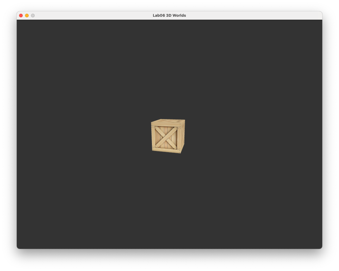
Run your program and you should see the following.

6.5.1. Changing the fov angle

The field of view angle determines how much of the view space we can see in the screen space where the larger the angle the more we can see. When we increase the field of view angle it appears to the user that our view is zooming out whereas a decrease has the effect of zooming in (this is used a lot in first person shooter games to model the effect of a pair of binoculars or a sniper scope).

Experiment with the affect of changing the field of view angle.

Fig. 6.11 \(fov = 15^\circ\)

Fig. 6.12 \(fov = 90^\circ\)

---

6.6. A camera class

Our render loop is starting to look a bit messy so we are going to create a Camera class to handle all operations relating to the calculation of the view and projection matrices. In the common/ folder there is a header file and code file called camera.hpp and camera.cpp which are currently empty. Enter the following code into camera.hpp.

#pragma once

#include <iostream>
#include <common/maths.hpp>

class Camera
{
public:
    // Projection parameters
    float fov    = Maths::radians(45.0f);
    float aspect = 1024.0f / 768.0f;
    float near   = 0.2f;
    float far    = 100.0f;

    // Camera vectors
    glm::vec3 eye;
    glm::vec3 target;
    glm::vec3 worldUp = glm::vec3(0.0f, 1.0f, 0.0f);

    // Transformation matrices
    glm::mat4 view;
    glm::mat4 projection;

    // Constructor
    Camera(const glm::vec3 eye, const glm::vec3 target);

    // Methods
    void calculateMatrices();
};

You should be familiar with class declarations by now. Here we have declared a Camera class with attributes of the floats for the projection parameters, glm vector objects for the camera vectors and glm matrix objects for the view and projection matrices.

In the camera.cpp file add the following code.

#include <common/camera.hpp>

Camera::Camera(const glm::vec3 Eye, const glm::vec3 Target)
{
    eye    = Eye;
    target = Target;
}

void Camera::calculateMatrices()
{
    // Calculate the view matrix
    view = Maths::lookAt(eye, target, worldUp);

    // Calculate the projection matrix
    projection = Maths::perspective(fov, aspect, near, far);
}

The Camera class constructor creates a camera object and instantiates the \(\mathbf{eye}\) and \(\mathbf{target}\) vectors using the values of the two glm::vec3 objects that are inputted. The calculateMatrices() method calculates the view and projection matrices. These both use functions from the Maths class which we haven’t yet defined so lets do this now. In the Maths class declare the following functions.

// View and projection matrices
static glm::mat4 lookAt(glm::vec3 eye, glm::vec3 target, glm::vec3 worldUp);
static glm::mat4 perspective( const float fov,  const float aspect,
                              const float near, const float far);

Then define these functions in the maths.cpp file.

glm::mat4 Maths::lookAt(glm::vec3 eye, glm::vec3 target, glm::vec3 worldUp)
{
    glm::vec3 front = glm::normalize(target - eye);
    glm::vec3 right = glm::normalize(glm::cross(front, worldUp));
    glm::vec3 up    = glm::cross(right, front);

    glm::mat4 view;
    view[0][0] = right.x, view[0][1] = up.x, view[0][2] = -front.x;
    view[1][0] = right.y, view[1][1] = up.y, view[1][2] = -front.y;
    view[2][0] = right.z, view[2][1] = up.z, view[2][2] = -front.z;
    view[3][0] = -glm::dot(eye, right);
    view[3][1] = -glm::dot(eye, up);
    view[3][2] =  glm::dot(eye, front);

    return view;
}

glm::mat4 Maths::perspective(const float fov,  const float aspect,
                             const float near, const float far)
{
    float top   = near * tan(fov / 2.0f);
    float right = aspect * top;

    glm::mat4 projection;
    projection[0][0] = near / right;
    projection[1][1] = near / top;
    projection[2][2] = -(far + near) / (far - near);
    projection[2][3] = -1.0f;
    projection[3][2] = -2.0f * far * near / (far - near);

    return projection;
}

So now we have a Camera class lets use it to calculate our view and projection matrices. First create a Camera object by entering the following code before the main() function.

// Create camera object
Camera camera(glm::vec3(1.0f, 1.0f, 1.0f), glm::vec3(0.0f, 0.0f, -2.0f));

Here we have placed the camera at \((1, 1, 1)\) pointing towards \((0, 0, -2)\) (the same as before). We then need to calculate the view and projection matrices just before we calculate the \(MV\!P\) matrix by adding the following code.

// Calculate view and projection matrices
camera.calculateMatrices();

The last thing we need to do is to use the view and projection matrices from the camera object when calculating the \(MV\!P\) matrix. Edit your code so that it looks like the following.

//Calculate the MVP matrix and send it to the vertex shader
glm::mat4 MVP = camera.projection * camera.view * model;

Compile and run your code to check that everything is working correctly. You can now comment out the codes used to calculate the view and projection matrices as this is no long used.

---

6.7. Multiple objects

The last thing we are going to do in this lab is to add some more cubes to our 3D world. We can do this by defining the position of each cube and then, in the render loop, we loop through each cube and calculate its model matrix, calculate the \(MV\!P\) matrix and then render the current cube. Add the following code to your program before the render loop.

// Cube positions
vec3 cubePositions[] = {
    vec3( 0.0f,  0.0f,  0.0f),
    vec3( 2.0f,  5.0f, -10.0f),
    vec3(-3.0f, -2.0f, -3.0f),
    vec3(-4.0f, -2.0f, -8.0f),
    vec3( 2.0f,  2.0f, -6.0f),
    vec3(-4.0f,  3.0f, -8.0f),
    vec3( 0.0f, -2.0f, -5.0f),
    vec3( 4.0f,  2.0f, -4.0f),
    vec3( 2.0f,  0.0f, -2.0f),
    vec3(-1.0f,  1.0f, -2.0f)
};

// Cube rotation angles
float angle[10];
for (unsigned int i = 0 ; i < 10 ; i++)
    cubeAngles[i] = Maths::radians(20.0f * i);

This creates two arrays of glm::vec3 objects: cubePositions that contain the co-ordinates of the centres of 10 cubes and cubeAngles that contains a rotation angle based on the loop variable i. In the render loop replace the code used to calculate the \(MV\!P\) matrix and render the cube with the following.

// Loop through cubes and draw each one
for (int i = 0; i < 10; i++)
{
    // Calculate the model matrix
    glm::mat4 translate = Maths::translate(cubePositions[i]);
    glm::mat4 scale     = Maths::scale(glm::vec3(0.5f, 0.5f, 0.5f));
    glm::mat4 rotate    = Maths::rotate(cubeAngles[i], glm::vec3(1.0f, 1.0f, 1.0f));
    glm::mat4 model     = translate * rotate * scale;

    // Calculate the MVP matrix
    glm::mat4 MVP = camera.projection * camera.view * model;

    // Send MVP matrix to the vertex shader
    glUniformMatrix4fv(glGetUniformLocation(shaderID, "MVP"), 1,
                       GL_FALSE, &MVP[0][0]);

    // Draw the triangles
    glBindBuffer(GL_ELEMENT_ARRAY_BUFFER, EBO);
    glDrawElements(GL_TRIANGLES, sizeof(indices) / sizeof(unsigned int),
                   GL_UNSIGNED_INT, 0);
}

Here we loop through each of the 10 cubes and calculate the model matrix using the cubePositions and cubeAngles vectors. We need to change the position of the camera so that we can see all of the cubes. Add the following code before the view and projection matrices are calculated.

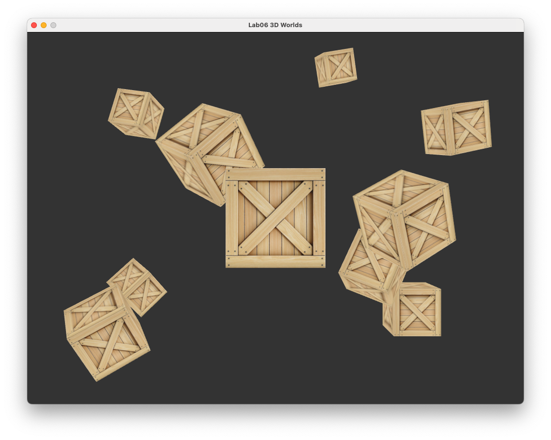
Camera camera(glm::vec3(0.0f, 0.0f, 5.0f), glm::vec3(0.0f, 0.0f, 0.0f));

This moves the camera position to \((0, 0, 5)\) looking towards \((0, 0, 0)\). Run your program and you should see the following.

---

6.8. Exercises

1. Move the camera position so that it moves in a circle centred at the first cube with radius 10 with a rotation speed such that it completes one full rotation every 5 seconds. Hint: \(x = c_x + r\cos(\theta)\) and \(z = c_z + r\sin(\theta)\) gives the \(x\) and \(y\) co-ordinates on a circle centred at \((c_x, c_y, c_z)\) with radius \(r\).

3. Rotate the cubes that have an odd index number about the vector \((1,1,1)\) so that they complete one full rotation every 2 seconds. Hint: x % y returns the remainder when x is divided by y, e.g., 3 % 2 will return 1.

4. Add a feature to your program that allows the user to increase or decrease the field of view angle using the up and down arrow keys. Your code should limit the field of view angle so it is never less than \(10^\circ\) or greater than \(90^\circ\). Hint: The keyboardInput() function at the bottom of the main.cpp file checks if the escape key has been pressed and quits the application if it has.