Lab 5: Transformations

Computer graphics requires that shapes are manipulated in space by moving the shapes, shrinking or stretching, rotating and reflection to name a few. We call these manipulations transformations. We need a convenient way of telling the computer how to apply our transformations and for this we make use of matrices which we covered in Lab 4: Vectors and Matrices.

Each transformation has an associated transformation matrix which we use to multiply the vertex coordinates of a shape to calculate the vertex coordinates of the transformed shape. For example if \(A\) is a transformation matrix for a particular transformation and \((x,y,z)\) are the coordinates of a vertex then we apply the transformation using

\[\begin{split} \begin{pmatrix} x' \\ y' \\ x' \end{pmatrix} = A \cdot \begin{pmatrix} x \\ y \\ z \end{pmatrix}, \end{split}\]

where \((x',y',z')\) are the coordinates of the transformed point. Note that all vectors and coordinates are written as a column vector when multiplying by a matrix.

Task

Create a folder called 05 Transformations and download index.html, transformations.js and webGLUtils.js to it. Open index.html in a web browser to check that the red triangle from Lab 3: Textures is displayed.

---

WebGL coordinate system

In 3D graphics a coordinate system defines how points, directions and rotations are represented. The two main conventions are the right-handed and left-handed coordinates systems. Both use \(x\), \(y\) and \(z\) axes but they differ in which direction the \(z\)-axis points relative to the \(x\) and \(y\) axis.

The right-handed coordinate system is where on your right hand:

• the thumb points along the positive \(x\)-axis,

• the index finger points along the positive \(y\)-axis,

• the middle finger points along the positive \(z\)-axis.

The other way of representing 3D space is to use a left-hand coordinate system which is the same but on your left hand.

WebGL uses the right-handed coordinate system where the \(x\)-axis points to the right of the screen, the \(y\)-axis points towards the top of the screen and the \(z\)-axis points out of the screen towards you (Fig. 30).

Fig. 30 The WebGL co-ordinate system.

Other graphics libraries that use the right-handed coordinate system include OpenGL, Three.js, Vulkan, Metal (Apple) and applications such as Unreal Engine and Blender. Graphics libraies that use the left-handed coordinate system include DirectX, Direct3D and Unity.

---

Translation

The translation transformation when applied to a set of points moves each point by the same amount. For example, consider the triangle in Fig. 31, each of the vertices has been translated by the same vector \(\vec{t}\) which has that effect of moving the triangle.

Fig. 31 Translation of a triangle by the translation vector \(\vec{t}= (t_x, t_y, t_z)\).

A problem we have is that no transformation matrix exists for applying translation to the coordinates \((x, y, z)\), i.e., we can’t find a matrix \(Translate\) such that

\[\begin{split}Translate \cdot \begin{pmatrix} x \\ y \\ z \end{pmatrix} = \begin{pmatrix} x + t_x \\ y + t_y \\ z + t_z \end{pmatrix}.\end{split}\]

We can use a trick where we use homogeneous coordinates. Homogeneous coordinates add another value, \(w\) say, to the \((x, y, z)\) coordinates (known as Cartesian coordinates) such that when the \(x\), \(y\) and \(z\) values are divided by \(w\) we get the Cartesian coordinates.

\[\begin{split} \underset{\textsf{homogeneous}}{\begin{pmatrix} x \\ y \\ z \\ w \end{pmatrix}} \equiv \underset{\textsf{Cartesian}}{\begin{pmatrix} x/w \\ y/w \\ z/w \end{pmatrix}}.\end{split}\]

So if we choose \(w=1\) then we can write the Cartesian coordinates \((x, y, z)\) as the homogeneous coordinates \((x, y, z, 1)\) (remember that 4-element vector with the additional 1 in our vertex shader?). So how does that help us with our elusive translation matrix? Well we can now represent translation as a \(4 \times 4\) matrix

\[\begin{split} \begin{pmatrix} 1 & 0 & 0 & t_x \\ 0 & 1 & 0 & t_y \\ 0 & 0 & 1 & t_z \\ 0 & 0 & 0 & 1 \end{pmatrix} \begin{pmatrix} x \\ y \\ z \\ 1 \end{pmatrix} = \begin{pmatrix} x + t_x \\ y + t_y \\ z + t_z \\ 1 \end{pmatrix},\end{split}\]

which is our desired translation. So the translation matrix for translating a set of points by the vector \(\vec{t} = (t_x, t_y, t_z)\) is

\[\begin{split}Translate = \begin{pmatrix} 1 & 0 & 0 & t_x \\ 0 & 1 & 0 & t_y \\ 0 & 0 & 1 & t_z \\ 0 & 0 & 0 & 1 \end{pmatrix}.\end{split}\]

Important

Recall that WebGL and glm use column-major order, so when coding transformation matrices into JavaScript we need to code the transpose of the matrix. So the translation matrix we are going to use is

(9)\[\begin{split}Translate = \begin{pmatrix} 1 & 0 & 0 & 0 \\ 0 & 1 & 0 & 0 \\ 0 & 0 & 1 & 0 \\ t_x & t_y & t_z & 1 \end{pmatrix}\end{split}\]

Let’s translate the rectangle \(0.4\) to the right and \(0.3\) upwards (remember we are dealing with normalised device coordinates, so the window coordinates are between \(-1\) and \(1\)). The transposed transformation matrix to perform this translation is

\[\begin{split} Translate = \begin{pmatrix} 1 & 0 & 0 & 0 \\ 0 & 1 & 0 & 0 \\ 0 & 0 & 1 & 0 \\ 0.4 & 0.3 & 0 & 1 \end{pmatrix}.\end{split}\]

We are going to define matrix class to compute the various transformation matrices.

Task

Add the following function definition to the matrix class in the maths.js file.

// Transformation matrices
translate(x, y, z) {
  return new Mat4().set(
    1, 0, 0, 0,
    0, 1, 0, 0,
    0, 0, 1, 0,
    x, y, z, 1
  );
}

And add the following to the translations.js file before we draw the triangles.

// Calculate transformation matrices
const translate = new Mat4().translate(0.4, 0.3, 0);

Here we have defined the function translate() that results the translation matrix for a given translation vector and have called this function to compute translateMatrix.

The multiplication of the vertex coordinates by the transformation matrices is done in the GPU as opposed to the CPU. This is because GPUs are specifically designed to perform matrix multiplication on millions of vertices in parallel, so doing this in the GPU is much faster and frees up the CPU. So we send the transformation matrix to the vertex shader using a uniform, like we did in the lab on texture maps.

Task

Add the following code after we have calculated the translation matrix.

// Calculate transformation matrix and send it to the shader
const model = translate;
gl.uniformMatrix4fv(gl.getUniformLocation(shaderProgram, "uModel"), false, model.m);

Here we have created another matrix called model and have sent this to the shader using the uniform name uModel. We will be applying multiple transformations to our object vertices. Rather then sending multiple matrices to the shaders, we multiply them in the CPU and send a single \(4 \times 4\) matrix to the shaders. The model matrix is the combination of transformations that are applied to each vertex of the object.

We now have to do is modify the vertex shader to use our new transformation matrix.

Task

In the vertex shader definition at the top of the transformations.js file, add the following uniform declaration before the main() function.

uniform mat4 uModel;

And change the calculation of gl_Position to the following

gl_Position = uModel * vec4(aPosition, 1.0);

Refresh your web browser and you should see that our rectangle has been translated to the right and up a bit as shown in Fig. 32.

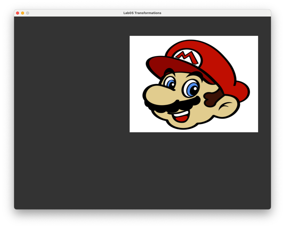
Fig. 32 The rectangle is translated by the vector \((0.4, 0.3, 0)\).

---

Scaling

Scaling is one of the simplest transformation we can apply. Multiplying the \(x\), \(y\) and \(z\) coordinates of a point by a scalar quantity (a number) has the effect of moving the point closer or further away from the origin (0,0). For example, consider the triangle in Fig. 33. The \(x\), \(y\) and \(z\) coordinates of each vertex has been multiplied by \(s_x\), \(s_y\) and \(s_y\) respectively which has the effect of scaling the triangle and moving the vertices further away from the origin (in this case because \(s_x\), \(s_y\) and \(s_z\) are all greater than 1).

Fig. 33 Scaling a triangle centred at the origin.

Since scaling is simply multiplying the coordinates by a number we have

\[\begin{split} \begin{align*} \begin{pmatrix} s_x & 0 & 0 & 0 \\ 0 & s_y & 0 & 0 \\ 0 & 0 & s_z & 0 \\ 0 & 0 & 0 & 1 \end{pmatrix} \begin{pmatrix} x \\ y \\ z \\ 1 \end{pmatrix} = \begin{pmatrix} s_xx \\ s_yy \\ s_zz \\ 1 \end{pmatrix}, \end{align*}\end{split}\]

so the scaling matrix for applying the scaling transformation is

(10)\[\begin{split} Scale = \begin{pmatrix} s_x & 0 & 0 & 0 \\ 0 & s_y & 0 & 0 \\ 0 & 0 & s_z & 0 \\ 0 & 0 & 0 & 1 \end{pmatrix}. \end{split}\]

Let’s now apply scaling to our rectangle in WebGL to increase its size by a factor of 0.5 in the horizontal direction and 0.4 in the vertical direction. The scaling matrix that achieves this is

\[\begin{split}Scale = \begin{pmatrix} 0.5 & 0 & 0 & 0 \\ 0 & 0.4 & 0 & 0 \\ 0 & 0 & 1 & 0 \\ 0 & 0 & 0 & 1 \end{pmatrix}.\end{split}\]

We have already created a model matrix and the uniform in the vertex shader, so we just need to calculate the scaling matrix and use it instead of the translation matrix.

Task

Enter the following function definition to the matrix class.

scale(x, y, z) {
  return new Mat4().set(
    x, 0, 0, 0,
    0, y, 0, 0,
    0, 0, z, 0,
    0, 0, 0, 1
  );
}

Enter the following code to the tranformations.js file after we calcuate the translation matrix.

const scale     = new Mat4().scale(0.5, 0.4, 1);

And change the model matrix to the following.

const model = scale;

Refresh your web browser and you should see that our rectangle has been scaled down as shown in Fig. 34.

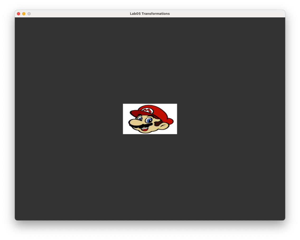
Fig. 34 The rectangle is scaled by the vector \((0.5, 0.4, 1)\).

Note

If scaling is applied to a shape that is not centred at \((0,0,0)\) then the transformed shape is distorted and its centre is moved from its original position (Fig. 35).

Fig. 35 Scaling applied to a triangle not centred at \((0,0,0)\).

If the desired result is to resize the shape whilst keeping its dimensions and location the same we first need to translate the vertex coordinates by \(-\vec{c}\) where \(\vec{c}\) is the centre of volume for the shape so that it is at \((0,0,0)\). Then we can apply the scaling before translating by \(\vec{c}\) so that the centre of volume is back at the original position (Fig. 36).

Fig. 36 The steps required to scale a shape about its centre.

---

Rotation

As well as translating and scaling objects, the next most common transformation is the rotation of objects around the three co-ordinate axes \(x\), \(y\) and \(z\). We define the rotation anti-clockwise around each of the co-ordinate axes by an angle \(\theta\) when looking down the axes (Fig. 37).

Fig. 37 Rotation is assumed to be in the anti-clockwise direction when looking down the axis.

The rotation matrices for achieving these rotations are

\[\begin{split} \begin{align*} R_x &= \begin{pmatrix} 1 & 0 & 0 & 0 \\ 0 & \cos(\theta) & -\sin(\theta) & 0 \\ 0 & \sin(\theta) & \cos(\theta) & 0 \\ 0 & 0 & 0 & 1 \end{pmatrix}, \\ R_y &= \begin{pmatrix} \cos(\theta) & 0 & \sin(\theta) & 0 \\ 0 & 1 & 0 & 0 \\ -\sin(\theta) & 0 & \cos(\theta) & 0 \\ 0 & 0 & 0 & 1 \end{pmatrix}, \\ R_z &= \begin{pmatrix} \cos(\theta) & -\sin(\theta) & 0 & 0 \\ \sin(\theta) & \cos(\theta) & 0 & 0 \\ 0 & 0 & 1 & 0 \\ 0 & 0 & 0 & 1 \end{pmatrix}. \end{align*} \end{split}\]

You don’t really need to know how these are derived but if you are curious you can click on the dropdown link below.

Derivation of the rotation matrices (click to show)

We will consider rotation about the \(z\)-axis and will restrict our coordinates to 2D.

Fig. 38 Rotating the vector \(\vec{a}\) anti-clockwise by angle \(\theta\) to the vector \(\vec{b}\).

Consider Fig. 38 where the vector \(\vec{a}\) is rotated by angle \(\theta\) to the vector \(\vec{b}\). If we form a right-angled triangle (the blue one) then we know the length of the hypotenuse, \(\|\vec{a}\|\), and the angle \(\theta\) so we can calculate the lengths of the adjacent and opposite sides using trigonometry. Remember our trig ratios (SOH-CAH-TOA)

\[\begin{align*} \sin(\phi) &= \frac{opposite}{hypotenuse}, & \cos(\phi) &= \frac{adjacent}{hypotenuse}, & \tan(\phi) &= \frac{opposite}{adjacent}, \end{align*}\]

so the length of the adjacent and opposite sides of the blue triangle is

\[\begin{split}\begin{align*} adjacent &= hypotenuse \cdot \cos(\phi), \\ opposite &= hypotenuse \cdot \sin(\phi). \end{align*}\end{split}\]

Since \(a_x\) and \(a_y\) are the lengths of the adjacent and opposite sides respectively and \(\|\vec{a}\|\) is the length of the hypotenuse we have

(11)\[\begin{split} \begin{align*} a_x &= \|\vec{a}\| \cos(\phi), \\ a_y &= \|\vec{a}\| \sin(\phi). \end{align*} \end{split}\]

Using the same method for the vector \(\vec{b}\) we have

(12)\[\begin{split} \begin{align*} b_x &= \|\vec{a}\| \cos(\phi + \theta), \\ b_y &= \|\vec{a}\| \sin(\phi + \theta). \end{align*} \end{split}\]

We can rewrite \(\cos(\phi+\theta)\) and \(\sin(\phi+\theta)\) using trigonometric identities

\[\begin{split}\begin{align*} \cos(\phi + \theta) &= \cos(\phi) \cos(\theta) - \sin(\phi) \sin(\theta), \\ \sin(\phi + \theta) &= \sin(\phi) \cos(\theta) + \cos(\phi) \sin(\theta), \end{align*}\end{split}\]

so equation (12) is

(13)\[\begin{split} \begin{align*} b_x &= \|\vec{a}\| \cos(\phi) \cos(\theta) - \|\vec{a}\| \sin(\phi) \sin(\theta), \\ b_y &= \|\vec{a}\| \sin(\phi) \cos(\theta) + \|\vec{a}\| \cos(\phi) \sin(\theta). \end{align*} \end{split}\]

Substituting equation (11) into equation (13) gives

\[\begin{split}\begin{align*} b_x &= a_x \cos(\theta) - a_y \sin(\theta), \\ b_y &= a_y \sin(\phi) + a_x \sin(\theta), \end{align*}\end{split}\]

which can be written using matrices as

\[\begin{split}\begin{align*} \begin{pmatrix} b_x \\ b_y \end{pmatrix} = \begin{pmatrix} \cos(\theta) & -\sin(\theta) \\ \sin(\theta) & \cos(\theta) \end{pmatrix} \begin{pmatrix} a_x \\ a_y \end{pmatrix}, \end{align*}\end{split}\]

so the transformation (non-transposed) matrix for rotating around the \(z\)-axis in 2D is

\[\begin{split}\begin{pmatrix} \cos(\theta) & -\sin(\theta) \\ \sin(\theta) & \cos(\theta) \end{pmatrix}.\end{split}\]

We need a \(4\times 4\) matrix to represent 3D rotation around the \(z\)-axis so we replace the 3rd and 4th row and columns with the 3rd and 4th row and column from the \(4\times 4\) identity matrix giving

\[\begin{split}R_z = \begin{pmatrix} \cos(\theta) & -\sin(\theta) & 0 & 0 \\ \sin(\theta) & \cos(\theta) & 0 & 0 \\ 0 & 0 & 1 & 0 \\ 0 & 0 & 0 & 1 \end{pmatrix}.\end{split}\]

The rotation matrices for the rotation around the \(x\) and \(y\) axes are derived using a similar process.

Lets rotate our original rectangle anti-clockwise about the \(z\)-axis by \(\theta = 45^\circ\). The transposed rotation matrix to do this is

\[\begin{split}Rotate = \begin{pmatrix} \cos(45^\circ) & \sin(45^\circ) & 0 & 0 \\ -\sin(45^\circ) & \cos(45^\circ) & 0 & 0 \\ 0 & 0 & 1 & 0 \\ 0 & 0 & 0 & 1 \end{pmatrix}.\end{split}\]

Note

Angles in JavaScript are always expressed in radians so we need to use the following to convert from degrees to radians

\[radians = degrees \times \frac{\pi}{180}\]

Task

Enter the following function definition to the matrix class.

rotateZ(rad) {
  const c = Math.cos(rad);
  const s = Math.sin(rad);
  return new Mat4().set(
    c,  s, 0, 0,
    -s, c, 0, 0,
    0,  0, 1, 0,
    0,  0, 0, 1
  );
}

Add the following to the transformations.js file after we calculate the scaling matrix

const angle     = 45 * Math.PI / 180;
const rotate    = new Mat4().rotate(0, 0, 1, angle);

And change the model matrix to the following.

const model = rotate;

Here we defined a function to the matrix class to calculate the rotation matrix. Refresh your web browser and you should see that our rectangle has been rotated \(45^\circ\) degrees in the anti-clockwise direction as shown in Fig. 39.

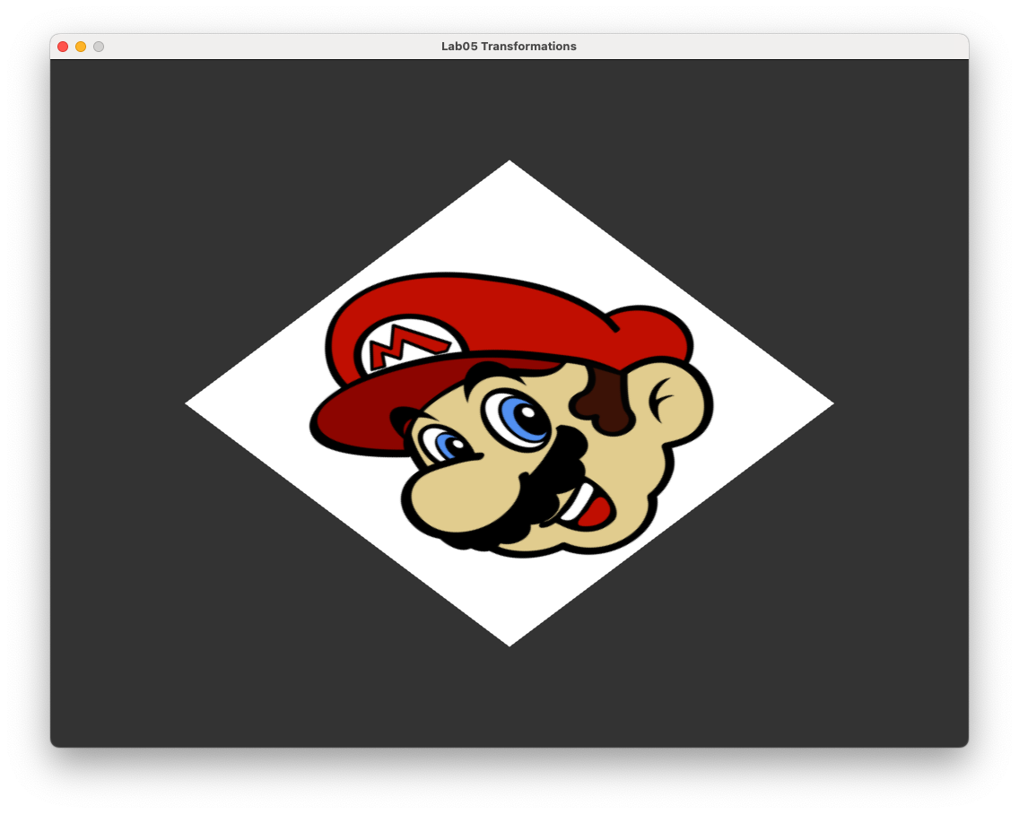
Fig. 39 Rectangle rotated anti-clockwise about the \(z\)-axis by \(45^\circ\).

---

Axis-angle rotation

The three rotation transformations are only useful if we want to only rotate around one of the three co-ordinate axes. A more useful transformation is the rotation around the axis that points in the direction of a unit vector \(\hat{v}\) which has its tail at \((0,0,0)\) (Fig. 40).

Fig. 40 Axis-angle rotation.

The transposed transformation matrix for rotation around a unit vector \(\hat{v} = (v_x, v_y, v_z)\), anti-clockwise by angle \(\theta\) when looking down the vector is.

(14)\[\begin{split} \begin{align*} Rotate = \begin{pmatrix} (1 - c) v_x^2 + c & (1 - c) v_x v_y + v_zs & (1 - c) v_x v_z - v_ys & 0 \\ (1 - c) v_x v_y - v_zs & (1 - c) v_y^2 + c & (1 - c) v_y v_z + v_xs & 0 \\ (1 - c) v_x v_z + v_ys & (1 - c) v_y v_z - v_xs & (1 - c) v_z^2 + c & 0 \\ 0 & 0 & 0 & 1 \end{pmatrix}. \end{align*} \end{split}\]

Where \(c = \cos(\theta)\) and \(s = \sin(\theta)\). Again, you don’t really need to know how this is derived but if you are curious click on the dropdown link below.

Derivation of the axis-angle rotation matrix (click to show)

The rotation about the unit vector \(\hat{v} = (v_x, v_y, v_z)\) by angle \(\theta\) is the composition of 5 separate rotations:

1. Rotate \(\hat{v}\) around the \(x\)-axis so that it is in the \(xz\)-plane (the \(y\) component of the vector is 0);

2. Rotate the vector around the \(y\)-axis so that it points along the \(z\)-axis (the \(x\) and \(y\) components are 0 and the \(z\) component is a positive number);

3. Perform the rotation around the \(z\)-axis;

4. Reverse the rotation around the \(y\)-axis;

5. Reverse the rotation around the \(x\)-axis.

---

1. The rotation around the \(x\)-axis is achieved by forming a right-angled triangle in the \(yz\)-plane where the the angle of rotation \(\theta\) has an adjacent side of length \(v_z\), an opposite side of length \(v_y\) and a hypotenuse of length \(\sqrt{v_y^2 + v_z^2}\) (Fig. 41).

Fig. 41 Rotate \(\vec{v}\) around the \(x\)-axis

Therefore \(\cos(\theta) = \dfrac{v_z}{\sqrt{v_y^2 + v_z^2}}\) and \(\sin(\theta) = \dfrac{v_y}{\sqrt{v_y^2 + v_z^2}}\) so the rotation matrix is

\[\begin{split}R_1 = \begin{pmatrix} 1 & 0 & 0 & 0 \\ 0 & \dfrac{v_z}{\sqrt{v_y^2 + v_z^2}} & -\dfrac{v_x}{\sqrt{v_y^2 + v_z^2}} & 0 \\ 0 & \dfrac{v_y}{\sqrt{v_y^2 + v_z^2}} & \dfrac{v_z}{\sqrt{v_y^2 + v_z^2}} & 0 \\ 0 & 0 & 0 & 1 \end{pmatrix}.\end{split}\]

---

2. The rotation around the \(y\)-axis is achieved by forming another right-angled triangle in the \(xz\)-plane where \(\theta\) has an adjacent side of length \(\sqrt{v_y^2 + v_z^2}\), an opposite side of length \(v_x\) and a hypotenuse of length 1 since \(\hat{v}\) is a unit vector (Fig. 42).

Fig. 42 Rotate around the \(y\)-axis

Therefore, \(\cos(\theta) = \sqrt{v_y^2 + v_z^2}\) and \(\sin(\theta) = v_x\). Note that here we are rotating in the clockwise direction so the rotation matrix is

\[\begin{split}R_2 = \begin{pmatrix} \sqrt{v_y^2 + v_z^2} & 0 & -v_x & 0 \\ 0 & 1 & 0 & 0 \\ v_x & 0 & \sqrt{v_y^2 + v_z^2} & 0 \\ 0 & 0 & 0 & 1 \end{pmatrix}.\end{split}\]

---

3. Now that the vector points along the \(z\)-axis we perform the rotation so the rotation matrix for this is

\[\begin{split}R_3 = \begin{pmatrix} \cos(\theta) & -\sin(\theta) & 0 & 0 \\ \sin(\theta) & \cos(\theta) & 0 & 0 \\ 0 & 0 & 1 & 0 \\ 0 & 0 & 0 & 1 \end{pmatrix}.\end{split}\]

---

4. The reverse rotation around the \(y\) is simply the rotation matrix \(R_2\) with the negative sign for \(\sin(\theta)\) swapped

\[\begin{split}\begin{align*} R_4 &= \begin{pmatrix} \sqrt{v_y^2 + v_z^2} & 0 & v_x & 0 \\ 0 & 1 & 0 & 0 \\ -v_x & 0 & \sqrt{v_y^2 + v_z^2} & 0 \\ 0 & 0 & 0 & 1 \end{pmatrix}. \end{align*}\end{split}\]

---

5. The reverse rotation around the \(x\) is simply the rotation matrix \(R_1\) with the negative sign for \(\sin(\theta)\) swapped

\[\begin{split}\begin{align*} R_5 &= \begin{pmatrix} 1 & 0 & 0 & 0 \\ 0 & \dfrac{v_z}{\sqrt{v_y^2 + v_z^2}} & \dfrac{v_y}{\sqrt{v_y^2 + v_z^2}} & 0 \\ 0 & -\dfrac{v_x}{\sqrt{v_y^2 + v_z^2}} & \dfrac{v_z}{\sqrt{v_y^2 + v_z^2}} & 0 \\ 0 & 0 & 0 & 1 \end{pmatrix}. \end{align*}\end{split}\]

---

Multiplying all the separate matrices together gives

\[\begin{split}\begin{align*} Rotate &= R_5 \cdot R_4 \cdot R_3 \cdot R_2 \cdot R_1 \\ &= \begin{pmatrix} \dfrac{v_x^2 + (v_y^2 + v_z^2)c}{\|\vec{v}\|^2} & \dfrac{v_xv_y(1 - c)}{\|\vec{v}\|^2} + \dfrac{v_zs}{\|\vec{v}\|} & \dfrac{v_xv_z(1 - c)}{\|\vec{v}\|^2} - \dfrac{v_ys}{\|\vec{v}\|} & 0 \\ \dfrac{v_xv_y(1 - c)}{\|\vec{v}\|^2} - \dfrac{v_zs}{\|\vec{v}\|} & \dfrac{v_y^2 + (v_x^2 + v_y^2)c}{\|\vec{v}\|^2} & \dfrac{v_yv_z(1 - c)}{\|\vec{v}\|^2} - \dfrac{v_xs}{\|\vec{v}\|} & 0 \\ \dfrac{v_xv_z(1 - c)}{\|\vec{v}\|^2} + \dfrac{v_ys}{\|\vec{v}\|} & \dfrac{v_yv_z(1 - c)}{\|\vec{v}\|^2} - \dfrac{v_xs}{\|\vec{v}\|} & \dfrac{v_z^2 + (v_x^2 + v_y^2)c}{\|\vec{v}\|^2} & 0 \\ 0 & 0 & 0 & 1 \end{pmatrix}. \end{align*}\end{split}\]

Where \(c = \cos(\theta)\) and \(s = \sin(\theta)\). Substituting \(v_y^2 + v_z^2 = 1 - v_x^2\) and the matrix simplifies to

\[\begin{split}\begin{align*} Rotate &= R_1 \cdot R_2 \cdot R_3 \cdot R_4 \cdot R_5 \\ &= \begin{pmatrix} (1 - c) v_x^2 + c & (1 - c) v_x v_y - v_zs & (1 - c) v_x v_z + v_ys & 0 \\ (1 - c) v_x v_y + v_zs & (1 - c) v_y^2 + c & (1 - c) v_y v_z - v_xs & 0 \\ (1 - c) v_x v_z - v_ys & (1 - c) v_y v_z + v_xs & (1 - c) v_z^2 + c & 0 \\ 0 & 0 & 0 & 1 \end{pmatrix}. \end{align*}\end{split}\]

Note that this matrix is transposed when we code it into JavaScript.

The rotations around the three coordinates axis can be calculated using the axis-angle rotation matrix (by letting \(\hat{v}\) be \((1,0,0)\), \((0,1,0)\) or \((0,0,1)\) for rotating around the \(x\), \(y\) and \(z\) axes respectively) so we can edit our rotate() function so that it uses equation (14).

Task

Edit the rotate() function in the maths.js file so that it looks like the following.

rotate(x, y, z, rad) {
 const len = Math.sqrt(x * x + y * y + z * z);
 if (len > 0) {
   x /= len; y /= len; z /= len;
 }
 const c = Math.cos(rad);
 const s = Math.sin(rad);
 const t = 1 - c;

 return new Mat4().set(
   t * x * x + c,      t * x * y + s * z,  t * x * z - s * y,  0,
   t * y * x - s * z,  t * y * y + c,      t * y * z + s * x,  0,
   t * z * x + s * y,  t * z * y - s * x,  t * z * z + c,      0,
   0, 0, 0, 1
 );
}

And change the calculation of the rotation matrix to the following

const rotate    = new Mat4().rotate(0, 0, 1, angle);

Here we have changed our function for calculating the rotation matrix so that it uses axis-angle rotation and have used it to rotate the rectangle by \(45^\circ\) anti-clockwise about a vector pointing along the \(z\)-axis (i.e., straight out of the screen towards you). Refreshing your browser and you should see that the output doesn’t change (Fig. 39).

---

Composite transformations

So far we have performed translation, scaling and rotation transformations on our rectangle separately. What if we wanted to combine these transformations so that we can control the size, rotation and position of the rectangle? If we apply the transformations in the order scale then rotate then translate then applying the scaling we have

\[\begin{split}\begin{align*} \begin{pmatrix} x' \\ y' \\ z' \\ 1 \end{pmatrix} &= Scale \cdot \begin{pmatrix} x \\ y \\ z \\ 1 \end{pmatrix}. \end{align*}\end{split}\]

Next applying rotation to the scaled coordinates we have

\[\begin{split}\begin{align*} \begin{pmatrix} x' \\ y' \\ z' \\ 1 \end{pmatrix} &= Rotate \cdot Scale \cdot \begin{pmatrix} x \\ y \\ z \\ 1 \end{pmatrix}. \end{align*}\end{split}\]

Finally applying translation to the scaled and rotated coordinates we have

\[\begin{split}\begin{align*} \begin{pmatrix} x' \\ y' \\ z' \\ 1 \end{pmatrix} &= Translate \cdot Rotate \cdot Scale \cdot \begin{pmatrix} x \\ y \\ z \\ 1 \end{pmatrix}. \end{align*}\end{split}\]

\(Translate \cdot Rotate \cdot Scale\) is a single \(4 \times 4\) transformation matrix that combines the three transformations known as the model matrix. Note the order that the translations are applied to the coordinates is read from right to left.

Lets apply scaling, rotation and translation (in that order) to our rectangle. Since we have already calculated the separate transformation matrices all we need to do is to multiply them together when calculating the model matrix.

Task

Change the model matrix to the following.

const model = translate.multiply(rotate).multiply(scale);

Refresh your web browser and you should see that the rectangle has been scaled down, rotated anti-clockwise and then translated as shown in Fig. 43.

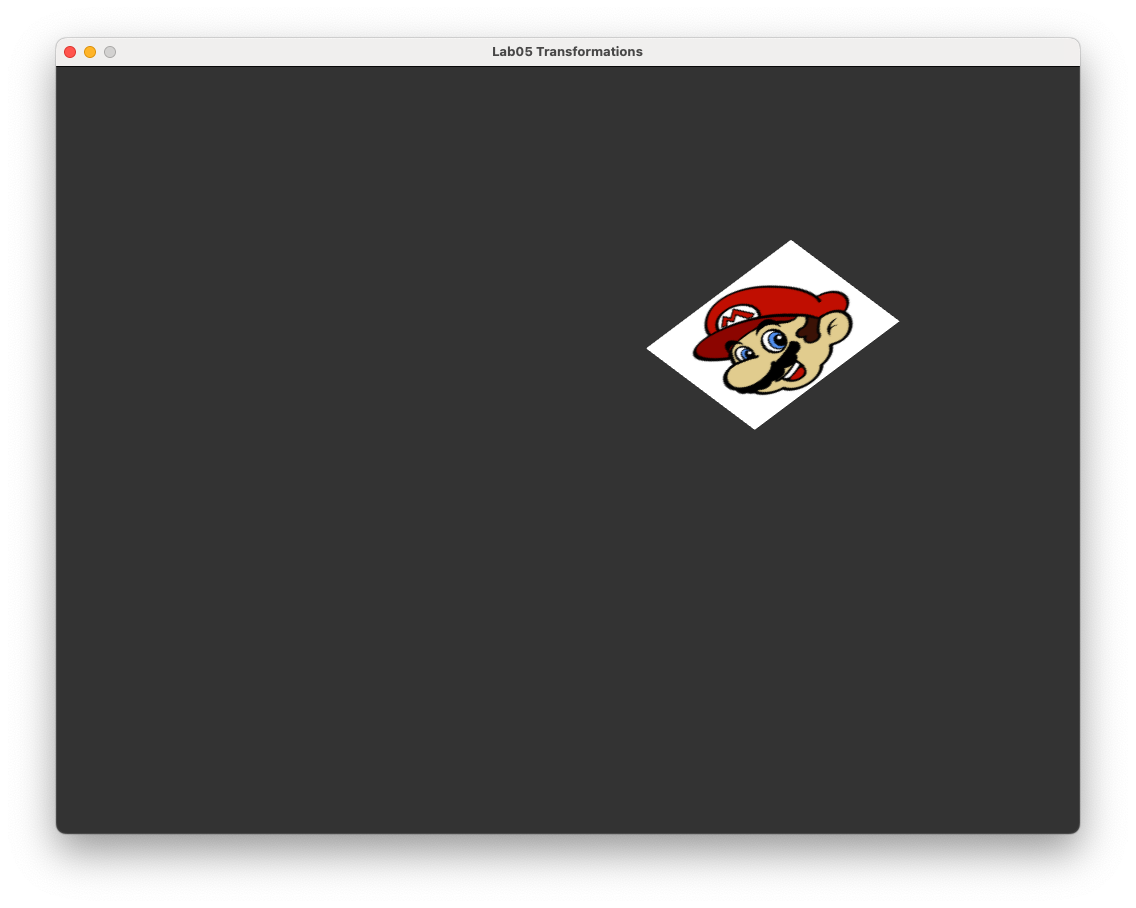
Fig. 43 Scaling, rotation and translation applied to the textured rectangle.

---

Animation

We are now going to introduce animation to our WebGL application so that we can better see the effects of animations. Animation is done by redrawing the scene while updating values that represent motion or change, such as the position and size of an object. In WebGL this is done using the brower’s built-in function

requestAnimationFrame(callback)

This schedules the rendering function to run before the next screen refresh (typically 60 times per second). The callback() function is used to update the animation state (e.g., move, scale, rotate objects), read input (e.g., from keyboad and mouse), set the shader uniforms (e.g., transformation matrices), and draw the frame. The callback recieves a timestamp that is the time in milliseconds since the rendering of the last frame which is useful for controlling movement speed.

We are going to make a few changes to our transformations.js file to animate the rectangle.

Task

First comment out (or delete) the code used to calculate the transformation matrices, the model matrix and sending the model matrix to the shader and also the draw commands (trust me).

Then add the following function definite to the transformations.js file before the main() function.

// Render frame
function render(time) {

  // Clear canvas
  gl.clear(gl.COLOR_BUFFER_BIT);

  // Calculate transformation matrices
  const translate = new Mat4().translate(0.4, 0.3, 0);
  const scale     = new Mat4().scale(0.5, 0.4, 1);
  const angle     = 1/2 * time * 0.001 * 2 * Math.PI;
  const rotate    = new Mat4().rotate(0, 0, 1, angle);

  // Calculate transformation matrix and send it to the shader
  const model = translate.multiply(rotate).multiply(scale);
  gl.uniformMatrix4fv(gl.getUniformLocation(shaderProgram, "uModel"), false, model.m);

  // Draw triangles
  gl.bindVertexArray(VAO);
  gl.drawElements(gl.TRIANGLES, 6, gl.UNSIGNED_SHORT, 0);

  // Call the render function before the next screen refresh
  requestAnimationFrame(render);
}

New add a call to this callback function at the end of the main() function

// Call the render function
render();

Here we have defined our callback function for the requestAnimationFrame() function. Note that this contains the code that you have deleted from the main() function and includes a call to requestAnimationFrame(render) which will re-render the frame when the browser is ready.

Refresh your web browser and you should see the same rectangle from Fig. 43. Although this may seem unimpressive, what is happening here is instead of rendering a single static frame, the canvas is being refreshed 60 times per second.

Let rotate our rectangle about its centre.

Task

Change the command used to calculate the rotation matrix to the following.

const angle     = 1/2 * time * 0.001 * 2 * Math.PI;
const rotate    = new Mat4().rotate(0, 0, 1, angle);

Here we calculate the rotation angle so that the rectangle will complete one full rotation every 2 seconds. Note that time is the time in milliseconds since the application was started hence we multiply the number of radians in a circle, \(2\pi\), by 0.001.

Refresh your browser and you should see something similar to below.

When calculating the composite transformation matrix the order in which we multiply the individual transformations will determine the effects of the composite transformation. To see this lets translate the rectangle first before rotating it.

Task

Change the calculation of the model matrix so that it looks like the following.

const model = rotate.multiply(translate).multiply(scale);

Here we have changed the order which the transformation matrices for translation and rotation are switched, i.e.,

\[Model = Rotate \cdot Translate \cdot Scale,\]

which has the effect of moving the rectangle so that it is centred at coordinates \((0.4, 0.3, 0)\) and then rotated about \((0, 0, 0)\). Refresh your browser and you should see something similar to below.

---

Exercises

1. Scale the original rectangle so that it is a quarter of the original size and apply translation so that the rectangle moves anti-clockwise around a circle centred at the window centre with radius 0.5 and completes one full rotation every 5 seconds. Hint: the coordinates of points on a circle centered at \((0,0)\) with radius \(r\) can be calculated using \(x = r\cos(t)\) and \(y = r\sin(t)\) where \(t\) is some number.

2. Rotate your rectangle from exercise 1 in a clockwise rotation about its centre at twice the rotation speed used in exercise 1.

3. Scale your rectangle from exercise 2 so that it grows and shrinks about its centre. Hint: The \(\sin(t)\) function oscillates between 0 and 1 as \(t\) increases.

4. Translate the rectangle so that it moves around the canvas and bounces off the borders.