Lab 9: Normal Mapping

In Lab 8: Lighting we saw that the diffuse and specular reflection models used the light source position and surface normal vector to determine the colour of a fragment. The vertex shader was used to interpolate the normal vectors for each fragment based on the normal vectors at the vertices of a triangle. This works well for smooth objects, but for objects with a rough or patterned surface we don’t get the benefits of highlights and shadow. Normal mapping is technique that uses a texture map to define the normal vectors for each fragment so that when a lighting model is applied it gives the appearance of a non-flat surface.

Fig. 92 Normal mapping applies a texture of normals for each fragment giving the appearance of a non-flat surface.

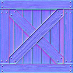
A normal map is a texture where the RGB colour values of each textel is used for the normal vector \(\vec{n} = (n_x, n_y, n_z)\) where \(n_x\), \(n_y\) and \(n_z\) values are determined by the red, green and blue colours values respectively. A normal map for the crate texture is shown in Fig. 93.

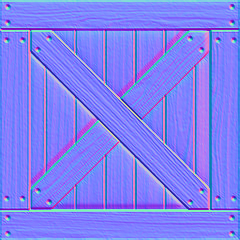
Fig. 93 A normal map for the crate texture.

Normal maps tend to have a blue tinge to them because the normal vectors are pointing away from the surface so the \(z\) component dominates. Any red on a normal map suggests that the normal is pointing to the right and green suggests the normal is pointing upwards.

Fig. 94 The RBG values of a normal map give the values of the normal vectors.

Task

Create a copy of your Lab 8 Lighting folder, rename it Lab 9 Normal Mapping, rename the file lighting.js to normal_mapping.js and change index.html so that the page title is “Lab 9 - Normal Maps” it embeds normal_mapping.js.

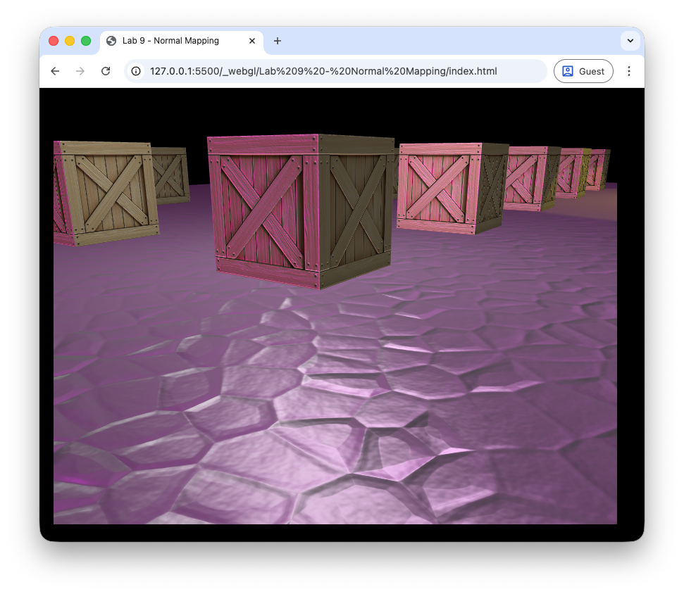
Load index.html in a live server, and you should see the cubes from Lab 8: Lighting lit using a point light, a spotlight and a directional light source.

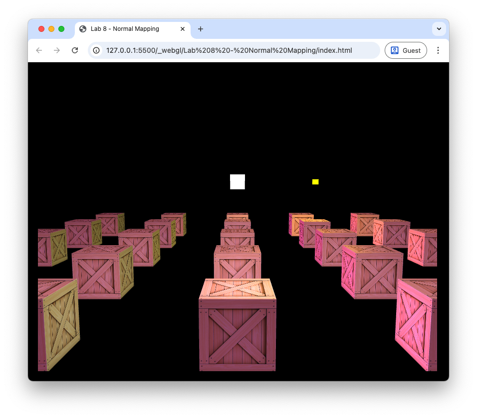
Fig. 95 The cubes lit using three light sources from Lab 8: Lighting.

Task

Download the file crate_normal.png and save it to the Lab 9 - Normal Mapping/assets/ folder.

In the normal_mapping.js file, add the following just after we have loaded the crate texture.

const normalMap = loadTexture(gl, "assets/crate_normal.png");

And add the following after we bind the crate texture in the render() function.

// Bind normal map
gl.activeTexture(gl.TEXTURE1);
gl.bindTexture(gl.TEXTURE_2D, normalMap);
gl.uniform1i(gl.getUniformLocation(program, "uNormalMap"), 1);

Here we have loaded the normal map for the crate texture and bind it to the sampler uNormalMap. Note that here we used the texture unit gl.TEXTURE1 which tells WebGL this is the second texture we are sending to the shaders (see Multiple textures).

---

Tangent space

We have already seen in Lab 6: 3D worlds that we can use transformations to map coordinates and vectors between the model, view and screen spaces. The normal vectors in a normal map are defined in tangent space, a local coordinate system aligned with the surface that has the basis vectors:

• Normal, \(\vec{N}\) - we have already met the normal vector which is a vector perpendicular to the surface.

• Tangent, \(\vec{T}\) - this is a vector that points in the direction of increasing texture coordinate \(u\).

• Bitangent, \(\vec{B}\) - this is a vector that points in the direction of increasing texture coordinate \(v\).

Fig. 96 The tangent space is defined by the tangent, bitangent and normal vectors.

The world space tangent vector \(\vec{T}\) is calculated using the model space vertex coordinates of the triangle \((x_0,y_0,z_0)\), \((x_1,y_1,z_1)\) and \((x_2,y_2,z_2)\) and their corresponding texture coordinates \((u_0,v_0)\), \((u_1,v_1)\) and \((u_2,v_2)\).

Fig. 97 The tangent, \(\vec{T}\), and bitangent, \(\vec{B}\), vectors are calculated by mapping the model space triangle onto the normal map space.

We first calculate vectors that point along two sides of the triangle in the model space

\[\begin{split} \begin{align*} \vec{e}_1 &= (x_1, y_1, z_1) - (x_0, y_0, z_0), \\ \vec{e}_2 &= (x_2, y_2, z_2) - (x_1, y_1, z_1), \end{align*}\end{split}\]

and calculate the difference in the \((u,v)\) coordinates for these edges

\[\begin{split} \begin{align*} \Delta u_1 &= u_1 - u_0, & \Delta v_1 &= v_1 - v_0, \\ \Delta u_2 &= u_2 - u_1, & \Delta v_2 &= v_2 - v_1. \end{align*} \end{split}\]

The tangent vector is then calculated using

(25)\[ \begin{align*} \vec{T} &= \frac{\Delta v_2 \cdot \vec{e}_1 - \Delta v_1 \cdot \vec{e}_2}{\Delta u_1\Delta v_2 - \Delta u_2\Delta v_1}. \end{align*} \]

To see the derivation of these equations click on the dropdown below.

Calculating the tangent and bitangent vectors

Consider Fig. 97 where a triangle is mapped onto the normal map using texture coordinates \((u_0,v_0)\), \((u_1,v_1)\) and \((u_2,v_2)\). If the vector \(\vec{T}\) and \(\vec{B}\) point in the \(u\) and \(v\) co-ordinate directions then the tangent space coordinates of points along the triangle edges \(\vec{e}_1\) and \(\vec{e}_2\) can be calculated using

\[\begin{split}\begin{align*} \vec{e}_1 &= \Delta u_1 \cdot \vec{T} + \Delta v_1 \cdot \vec{B}, \\ \vec{e}_2 &= \Delta u_2 \cdot \vec{T} + \Delta v_2 \cdot \vec{B}, \end{align*}\end{split}\]

where \(\Delta u_1 = u_1 - u_0\), \(\Delta v_1 = v_1 - v_0\), \(\Delta u_2 = u_2 - u_1\) and \(\Delta v_2 = v_2 - v_1\). We can express this using matrices

\[\begin{split} \begin{align*} \begin{pmatrix} \vec{e}_1 \\ \vec{e}_2 \end{pmatrix} &= \begin{pmatrix} \Delta u_1 & \Delta v_1 \\ \Delta u_2 & \Delta v_2 \end{pmatrix} \begin{pmatrix} \vec{T} \\ \vec{B} \end{pmatrix}. \end{align*} \end{split}\]

We want to calculate \(\vec{T}\) and \(\vec{B}\) and we know the values of \(\vec{e}_1\), \(\vec{e}_2\), \(\Delta u_1\), \(\Delta v_1\), \(\Delta u_2\) and \(\Delta v_2\). Using the inverse of the square matrix we can rewrite this equation as

\[\begin{split} \begin{align*} \begin{pmatrix} \vec{T} \\ \vec{B} \end{pmatrix} &= \begin{pmatrix} \Delta u_1 & \Delta v_1 \\ \Delta u_2 & \Delta v_2 \end{pmatrix}^{-1} \begin{pmatrix} \vec{e}_1 \\ \vec{e}_2 \end{pmatrix} \\ &= \frac{1}{\Delta u_1\Delta v_2 - \Delta u_2\Delta v_1} \begin{pmatrix} \Delta v_2 & -\Delta v_1 \\ -\Delta u_2 & \Delta u_1 \end{pmatrix} \begin{pmatrix} \vec{e}_1 \\ \vec{e}_2 \end{pmatrix}. \end{align*} \end{split}\]

Writing this out for the \(\vec{T}\) vector we have

\[ \begin{align*} \vec{T} &= \frac{\Delta v_2 \cdot \vec{e}_1 - \Delta v_1 \cdot \vec{e}_2}{\Delta u_1\Delta v_2 - \Delta u_2\Delta v_1}. \end{align*} \]

Since the bitangent vector \(\vec{B}\) is perpendicular to the normal vector \(\vec{N}\) and the tangent vector \(\vec{T}\) we can calculate this using

\[ \vec{B} = \vec{N} \times \vec{T}. \]

Once we have the tangent, bitangent and normal vectors we can form a matrix that transforms from the tangent space to the world space. The matrix that achieves this a 3 \(\times\) 3 matrix known as the \(TBN\) matrix

(26)\[\begin{split} \begin{align*} TBN &= \begin{pmatrix} \vec{T}_x & \vec{B}_x & \vec{N}_x \\ \vec{T}_y & \vec{B}_y & \vec{N}_y \\ \vec{T}_z & \vec{B}_z & \vec{N}_z \end{pmatrix}, \end{align*} \end{split}\]

Calculating the tangent vectors

All the lighting calculations are performed by the shaders, so we calculate the tangent vectors in JavaScript and pass them to the shaders using uniforms.

Task

Add the following function to the webGLUtils.js file.

function computeTangents(vertices, indices) {

  const stride = 11; // number of floats per vertex
  const vertexCount = vertices.length / stride;
  const tangents = new Float32Array(vertexCount * 3);

  for (let i = 0; i < indices.length; i += 3) {

    const i0 = indices[i];
    const i1 = indices[i + 1];
    const i2 = indices[i + 2];
    const v0 = i0 * stride;
    const v1 = i1 * stride;
    const v2 = i2 * stride;

    // Positions
    const p0x = vertices[v0 + 0];
    const p0y = vertices[v0 + 1];
    const p0z = vertices[v0 + 2];
    const p1x = vertices[v1 + 0];
    const p1y = vertices[v1 + 1];
    const p1z = vertices[v1 + 2];
    const p2x = vertices[v2 + 0];
    const p2y = vertices[v2 + 1];
    const p2z = vertices[v2 + 2];

    // UV coordinates
    const uv0x = vertices[v0 + 6];
    const uv0y = vertices[v0 + 7];
    const uv1x = vertices[v1 + 6];
    const uv1y = vertices[v1 + 7];
    const uv2x = vertices[v2 + 6];
    const uv2y = vertices[v2 + 7];

    // Edge vectors
    const e1x = p1x - p0x;
    const e1y = p1y - p0y;
    const e1z = p1z - p0z;
    const e2x = p2x - p0x;
    const e2y = p2y - p0y;
    const e2z = p2z - p0z;

    // UV deltas
    const du1 = uv1x - uv0x;
    const dv1 = uv1y - uv0y;
    const du2 = uv2x - uv0x;
    const dv2 = uv2y - uv0y;

    const denom = du1 * dv2 - du2 * dv1;
    if (Math.abs(denom) < 1e-6) continue;

    const f = 1.0 / denom;
    const tx = f * (dv2 * e1x - dv1 * e2x);
    const ty = f * (dv2 * e1y - dv1 * e2y);
    const tz = f * (dv2 * e1z - dv1 * e2z);

    // Accumulate tangent
    tangents[i0 * 3 + 0] += tx;
    tangents[i0 * 3 + 1] += ty;
    tangents[i0 * 3 + 2] += tz;

    tangents[i1 * 3 + 0] += tx;
    tangents[i1 * 3 + 1] += ty;
    tangents[i1 * 3 + 2] += tz;

    tangents[i2 * 3 + 0] += tx;
    tangents[i2 * 3 + 1] += ty;
    tangents[i2 * 3 + 2] += tz;
  }

  // Normalize tangents
  for (let i = 0; i < vertexCount; i++) {

    const tx = tangents[i * 3 + 0];
    const ty = tangents[i * 3 + 1];
    const tz = tangents[i * 3 + 2];

    const length = Math.sqrt(tx * tx + ty * ty + tz * tz);
    if (length > 0.0) {
      tangents[i * 3 + 0] /= length;
      tangents[i * 3 + 1] /= length;
      tangents[i * 3 + 2] /= length;
    }
  }

  return tangents;
}

Then, add the following to the createVao() function before we unbind the VAO.

// Tangents
const tangents = computeTangents(vertices, indices);
const tangentLocation = gl.getAttribLocation(program, "aTangent");
const tangentBuffer = gl.createBuffer();

gl.bindBuffer(gl.ARRAY_BUFFER, tangentBuffer);
gl.bufferData(gl.ARRAY_BUFFER, tangents, gl.STATIC_DRAW);
gl.enableVertexAttribArray(tangentLocation);
gl.vertexAttribPointer(tangentLocation, 3, gl.FLOAT, false, 0, 0);

Here we have written a function to compute the tangent vectors in the model space using equation (25), created a buffer for the tangents and sent it to the GPU simiarly to what we did for the vertex coordinates, texture coordinates and normal vectors.

---

Shaders

In the vertex shader we need to calculate the world space tangent and bitangent vectors for the vertex and output this to the fragment shader.

Task

Add input and output declarations to the vertex shader in the normal_mapping.js file.

in vec3 aTangent;


out vec3 vTangent;
out vec3 vBitangent;

Then add the following to the main() function

// Output world space tangent and bitangent vectors
vTangent = normalize(mat3(uModel) * aTangent);
vBitangent = normalize(cross(vNormal, vTangent));

Here we transform the tangent to the world space using the model matrix and calculate the bitangent vector using the cross product between the normal and tangent vectors. Now we need to edit the fragment shader to calculate the \(TBN\) matrix using equation (26) and use it to transform the normal vectors from the normal map from the tangent space to the world space.

The values in a texture are between 0 and 1, and we need the values of a normal vector to be between -1 and 1. So to convert the normal map colours to a tangent space normal vector we use the following

\[ \vec{n}_{tangent} = 2 \cdot \vec{n}_{map} - 1. \]

which is then transformed to the world space using

\[ \vec{n}_{world} = TBN \cdot \vec{n}_{tangent}. \]

Task

Add the following input declaration to the fragment shader.

in vec3 vTangent;
in vec3 vBitangent

And add the uniform for the normal map.

uniform sampler2D uNormalMap;

Then in the main() function, add the following before we calculate the lighting for each light source

// Calculate TBN matrix
mat3 TBN = mat3(normalize(vTangent), normalize(vBitangent), N);

// Calculate world space normal
vec3 normalSample = texture(uNormalMap, vTexCoords).rgb * 2.0 - 1.0;
N = normalize(TBN * normalSample);

Refresh your web browser and move the camera around to see the effects of the normal map.

Fig. 98 The crate normal map applied to the cubes.

The lighting properties of our cubes makes the surfaces look shiny. Since these should be wooden, we can reduce the specular coefficient to give a more realistic result.

Task

Change the ks attribute of the cube objects to the following.

ks        : 0.2,

Refresh your web browser and you should see that the cubes are now less shiny and more realistic.

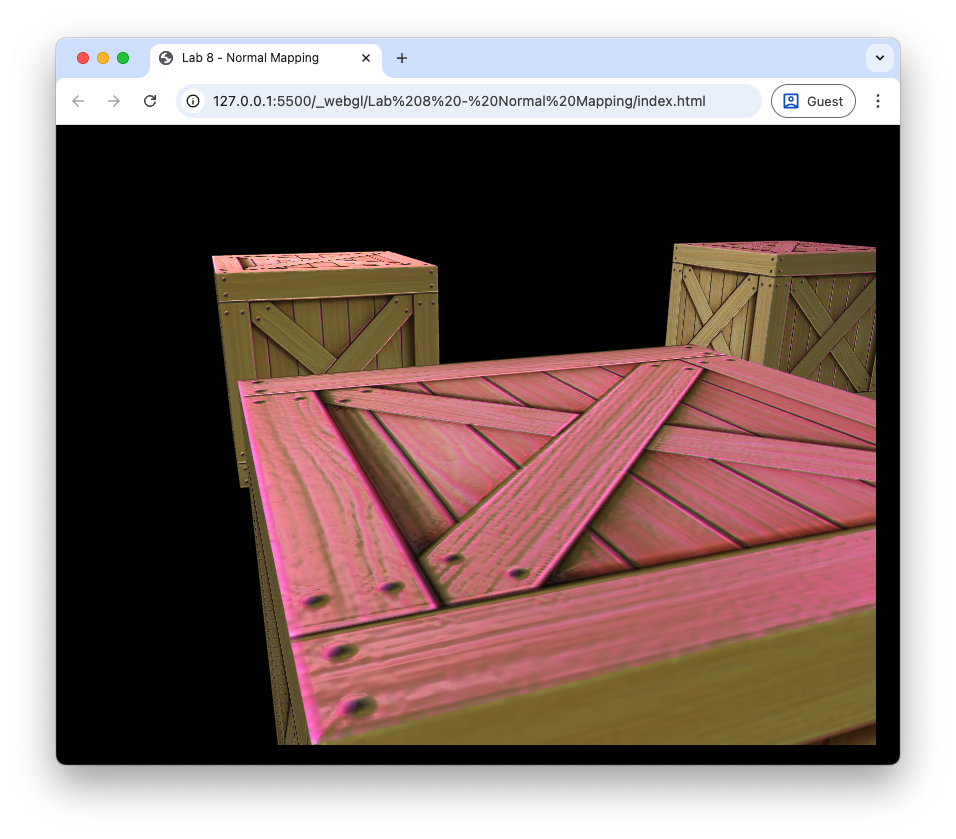
Fig. 99 The crate normal map applied to the cubes (\(k_s = 0.2\)).

Compare this to the non-normal mapped cubes and you can see the difference that normal mapping has made.

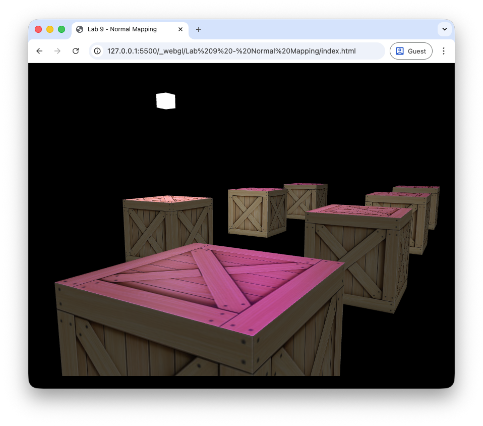
Fig. 100 Non-normal mapped cubes.

---

Specular maps

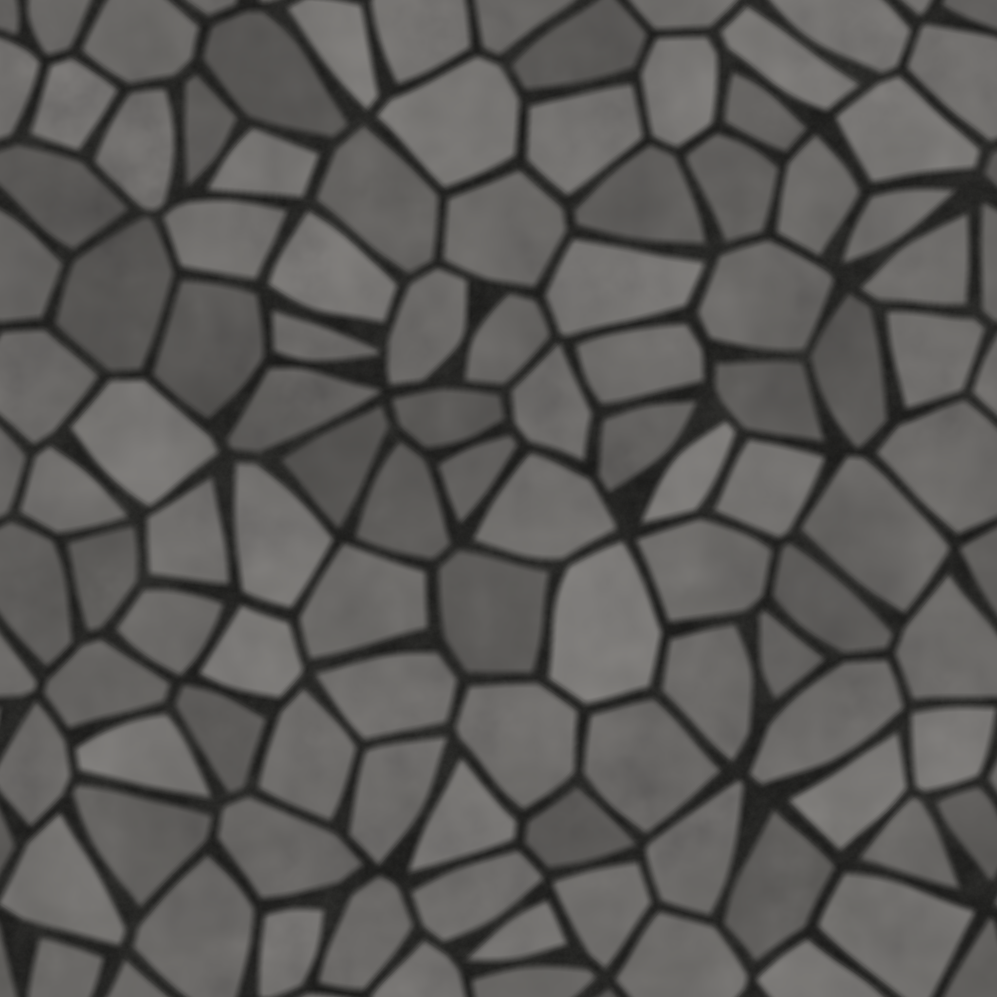
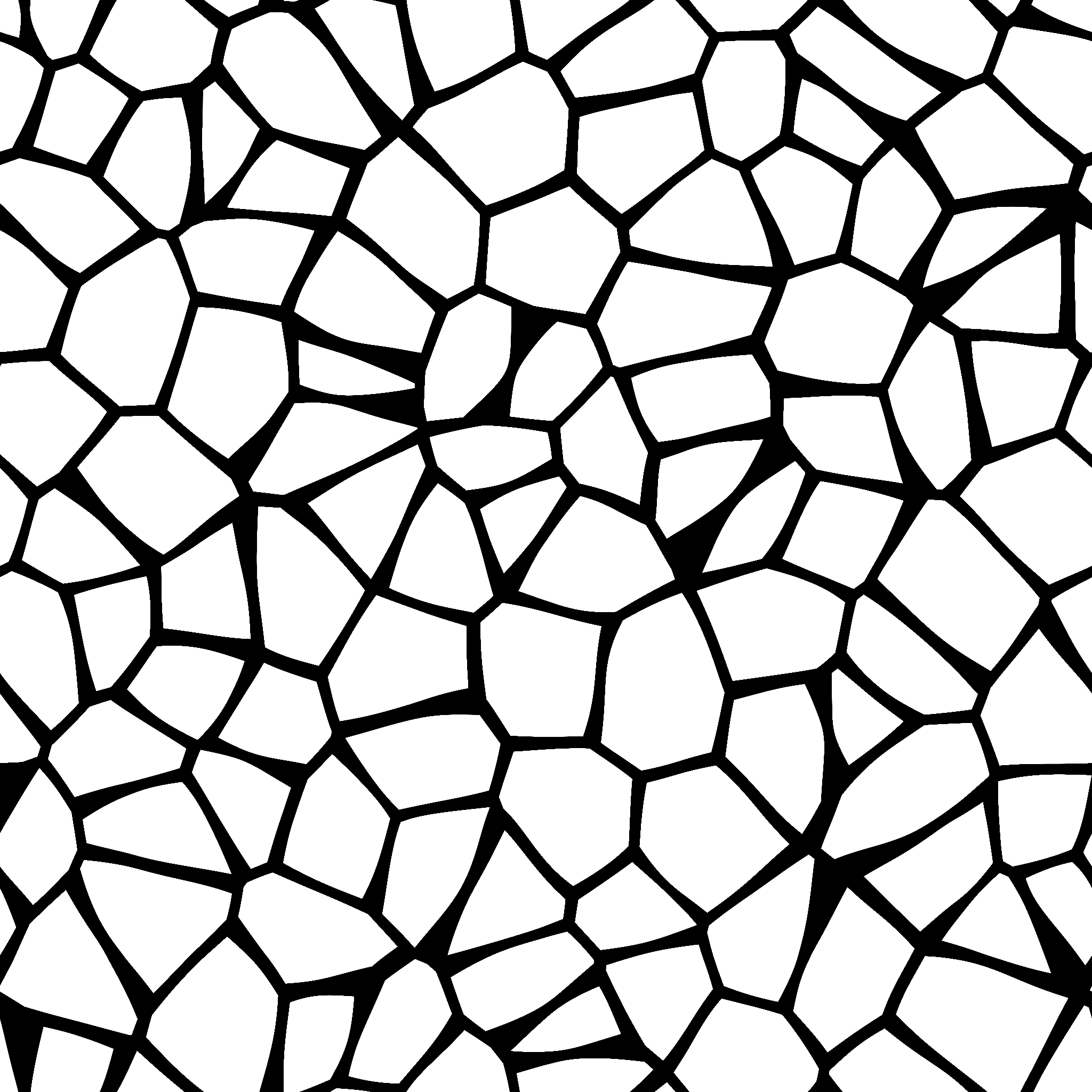
In addition to diffuse (texture) and normal maps we can also apply a specular map which can be used to control the specular highlights across a surface. Lets say we want to add a stone floor to our scene. We can add a horizontal polygon object for the floor and use a texture map Fig. 101 to give the impression of stones and a normal map Fig. 102 so that the stones are lit by the light sources.

Fig. 101 Diffuse map

Fig. 102 Normal map

Fig. 103 Specular map

To add our stone floor we are going to load in a simple 2D plane model, add diffuse and normal textures, define lighting and world space properties and draw it.

Task

Download the files stones.png and stones_normal.png and save them in your Lab 9 - Normal Mapping/assets/ folder.

Add the following code after we load the crate textures.

// Define floor vertices
const floorVertices = new Float32Array([
  // x y   z     R  G  B     u  v     nx  ny  nz
  -1,  0,  1,    0, 0, 0,    0, 0,    0,  1,  0,
   1,  0,  1,    0, 0, 0,    8, 0,    0,  1,  0,
   1,  0, -1,    0, 0, 0,    8, 8,    0,  1,  0,
  -1,  0, -1,    0, 0, 0,    0, 8,    0,  1,  0,
]);

// Define floor indices
const floorIndices = new Uint16Array([
  0,  1,  2,  
  0,  2,  3,
]);

// Define floor VAO
const floorVao = createVao(gl, program, floorVertices, floorIndices);

// Load floor textures
const floorTexture = loadTexture(gl, "assets/stones.png");
const floorNormalMap = loadTexture(gl, "assets/stones_normal.png");

And add the following after we have drawn the cubes.

// Draw floor
// Bind texture
gl.activeTexture(gl.TEXTURE0);
gl.bindTexture(gl.TEXTURE_2D, floorTexture);
gl.uniform1i(gl.getUniformLocation(program, "uTexture"), 0);

// Bind normal map
gl.activeTexture(gl.TEXTURE1);
gl.bindTexture(gl.TEXTURE_2D, floorNormalMap);
gl.uniform1i(gl.getUniformLocation(program, "uNormalMap"), 1);

// Send object light properties to the shader
gl.uniform1f(gl.getUniformLocation(program, "uKa"), 0.2);
gl.uniform1f(gl.getUniformLocation(program, "uKd"), 0.7);
gl.uniform1f(gl.getUniformLocation(program, "uKs"), 1.0);
gl.uniform1f(gl.getUniformLocation(program, "uShininess"), 32);

// Calculate the model matrix
const model = new Mat4()
  .translate([6, -0.5, -6])
  .scale([10, 1, 10]);
gl.uniformMatrix4fv(gl.getUniformLocation(program, "uModel"), false, model.m);

// Draw the triangles
gl.bindVertexArray(floorVao);
gl.drawElements(gl.TRIANGLES, floorIndices.length, gl.UNSIGNED_SHORT, 0);

Here we have added another object ot our scene that consists of a simple flat plane which has been scaled up and translated so that it forms a floor underneath the cubes. All of the this code is similar to what we have done previously. Refresh your web browser and move the camera around to see the effect of normal mapping on the stone floor.

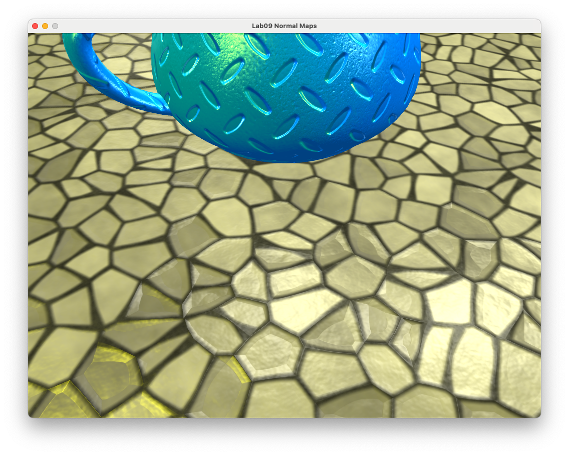
Fig. 104 A the floor object with normal mapping.

Note how the mortar between the stones have specular highlights. This isn’t very realistic as in real life mortar is rough and does not appear shiny. To overcome this we can apply a specular map (Fig. 103) to switch off the specular highlights for certain fragments.

Task

Download the file stones_specular.png and save it in your Lab 9 - Normal Mapping/assets/ folder.

Add the following code after we have loaded the floor textures.

const floorSpecularMap = loadTexture(gl, "assets/stones_specular.png");

And add the following after we bind the normal map for the floor.

// Bind specular map
gl.activeTexture(gl.TEXTURE2);
gl.bindTexture(gl.TEXTURE_2D, floorSpecularMap);
gl.uniform1i(gl.getUniformLocation(program, "uSpecularMap"), 2);

Then in the fragment shader, add a declaration for the specular map

uniform sampler2D uSpecularMap;

And add the following after the specular lighting is calculated.

specular *= texture(uSpecularMap, vTexCoords).rgb;

Refresh your web browser and position the camera to see the effect of the specular map. Note how the mortar between the stones no longer appears to be shiny.

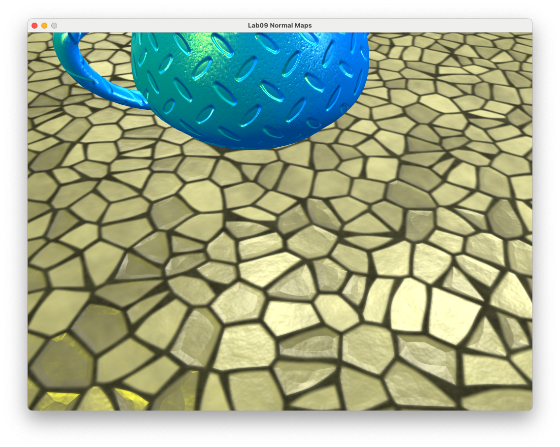
Fig. 105 A the floor object with normal and specular mapping.

Texture Map Flags

A problem we now have is that we hand bound a specular map for the floor object but this has also been applied to the cube objects.

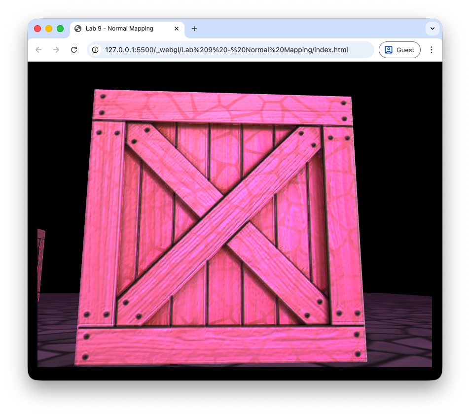
Fig. 106 The floor specular map has been applied to the cube objects.

To overcome this we can use a uniform boolean flag in the fragment shader that tells it whether a texture exists and use these to only apply the texture, normal or specular maps when they do.

Task

In the fragment shader, add uniforms for the texture flags

uniform bool uHasDiffuseMap;
uniform bool uHasNormalMap;
uniform bool uHasSpecularMap;

In the main() function, change the object colour to only use a texture (diffuse) map if it exists

// Object colour
vec4 objectColour = vec4(vColour, 1.0);
if (uHasDiffuseMap) {
  objectColour = texture(uTexture, vTexCoords);
}

and only apply a normal map if it exists

// Apply normal map
if (uHasNormalMap) {
  vec3 T = normalize(vTangent);
  vec3 B = cross(N, T);
  mat3 TBN = mat3(T, B, N);

  vec3 normalSample = texture(uNormalMap, vTexCoords).rgb * 2.0 - 1.0;
  N = normalize(TBN * normalSample);
}

In the computeLighting() function, only apply the specular map if it exists

// Apply specular map only if defined
if (uHasSpecularMap) {
  specular *= texture(uSpecularMap, vTexCoords).rgb;
}

Finally, send the texture flags for the cube objects after we bind their textures

// Send texture flags to the shader
gl.uniform1i(gl.getUniformLocation(program, "uHasDiffuseMap"), true);
gl.uniform1i(gl.getUniformLocation(program, "uHasNormalMap"), true);
gl.uniform1i(gl.getUniformLocation(program, "uHasSpecularMap"), false);

and do the same for the floor object

// Send texture flags to the shader
gl.uniform1i(gl.getUniformLocation(program, "uHasDiffuseMap"), true);
gl.uniform1i(gl.getUniformLocation(program, "uHasNormalMap"), true);
gl.uniform1i(gl.getUniformLocation(program, "uHasSpecularMap"), true);

Here we have set the specular map flag to false for the cube object but true for the floor object. Now when we look closely at the cube objects we no longer see the floor specular map being applied.

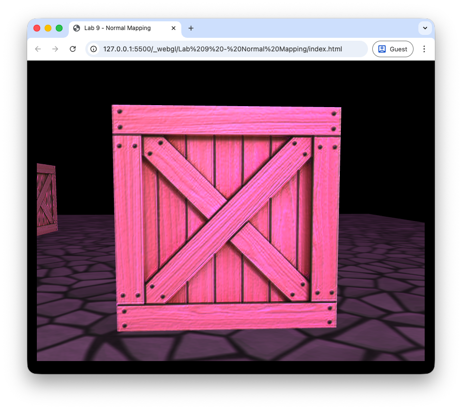
Fig. 107 The floor specular map is no longer being applied to the cube objects.

---

Exercises

1. (a) Change the diffuse texture of the floor object to that is uses a plain grey texture map based on the file grey.png.

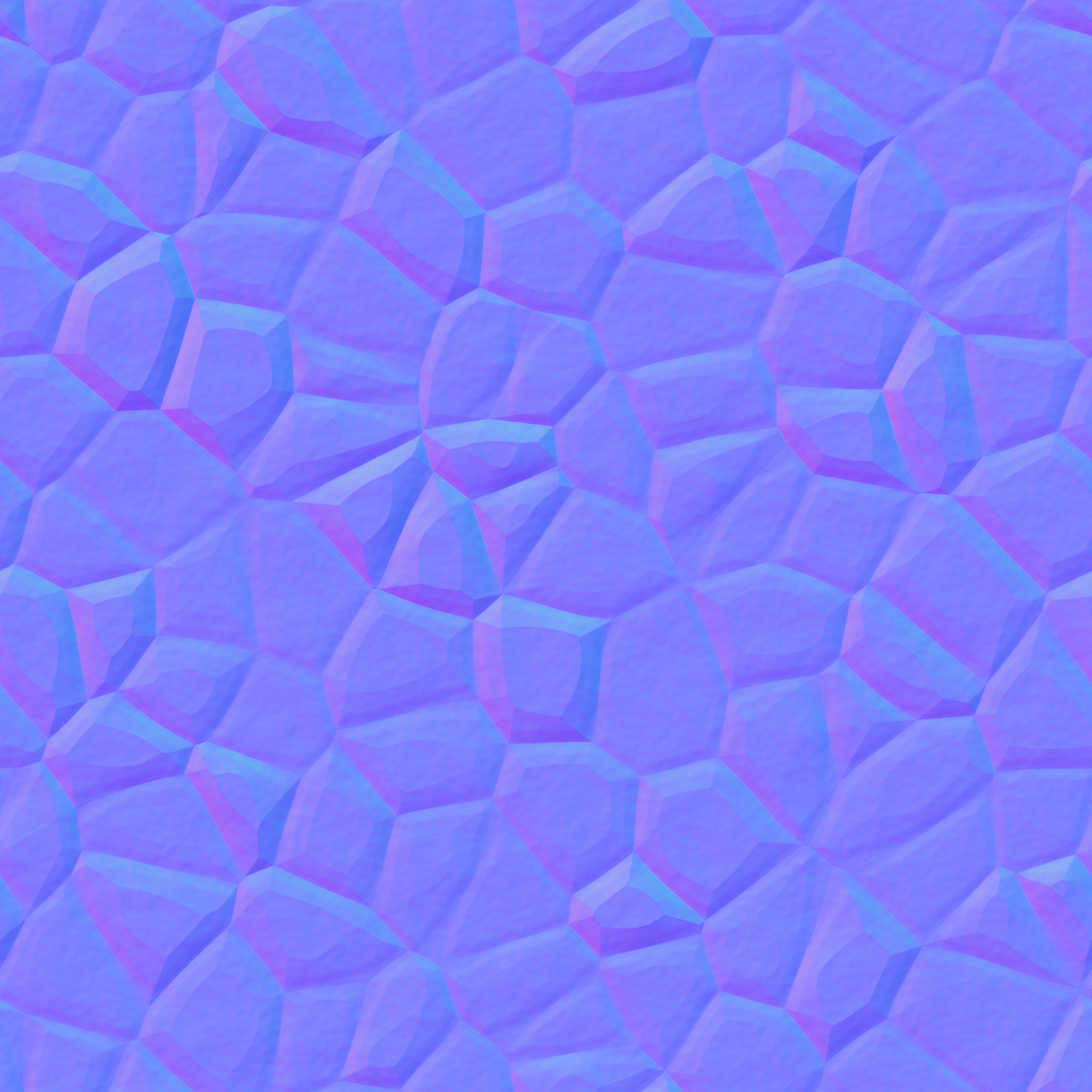
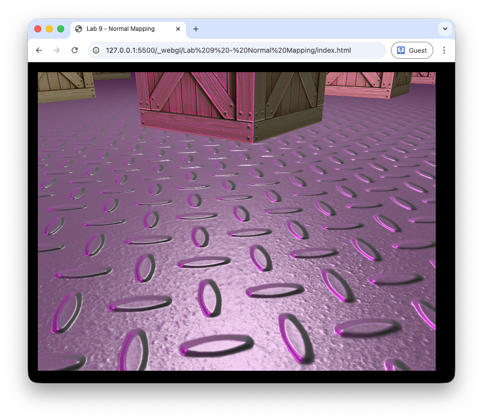
  (b) Change the normal map of the floor object to a diamond plate normal map based on the file diamond_normal.png. Set the texture co-ordinates of the floor object so that the textures are repeated four times in both \((u, v)\) directions.

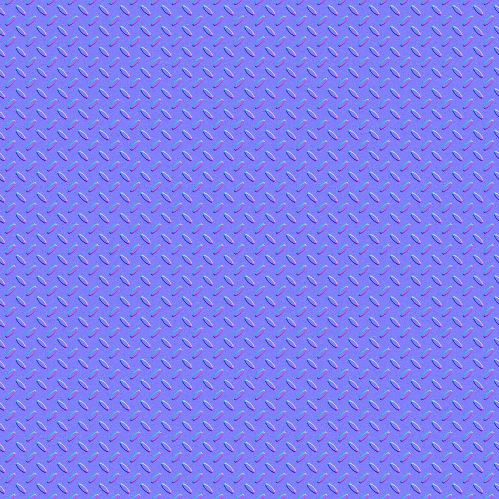
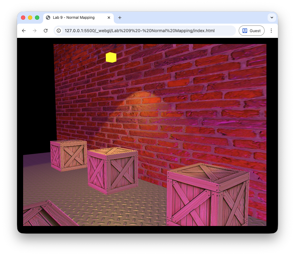
2. Add a brick wall object to your scene by doing the following:

  (a) Add another cube object that is scaled up using the scaling vector \(\vec{s} = (1, 4, 10)\) and translated by \(\vec{t} = (11, 3.5, -6)\).

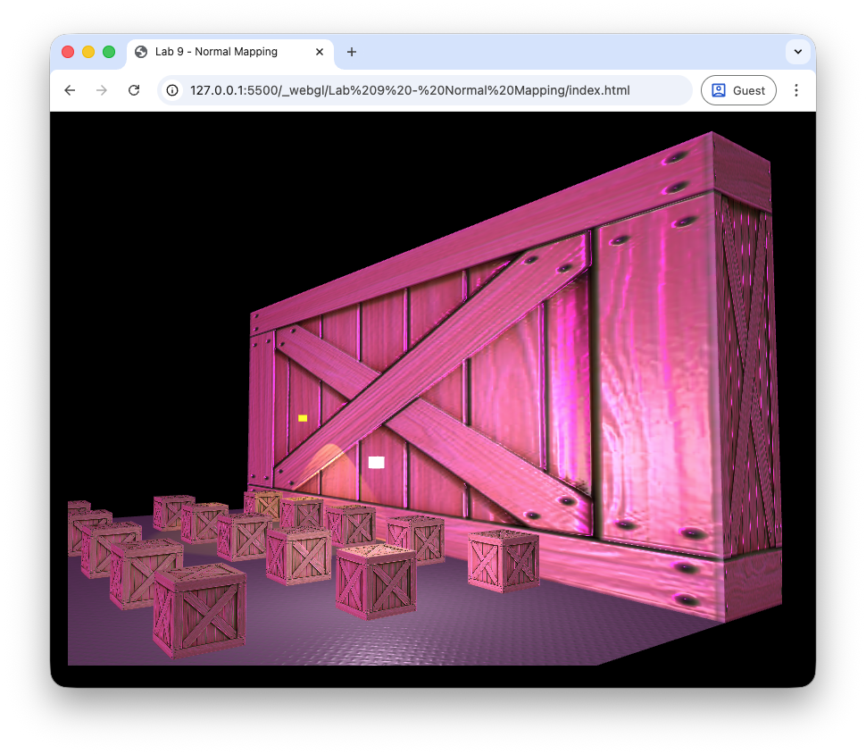
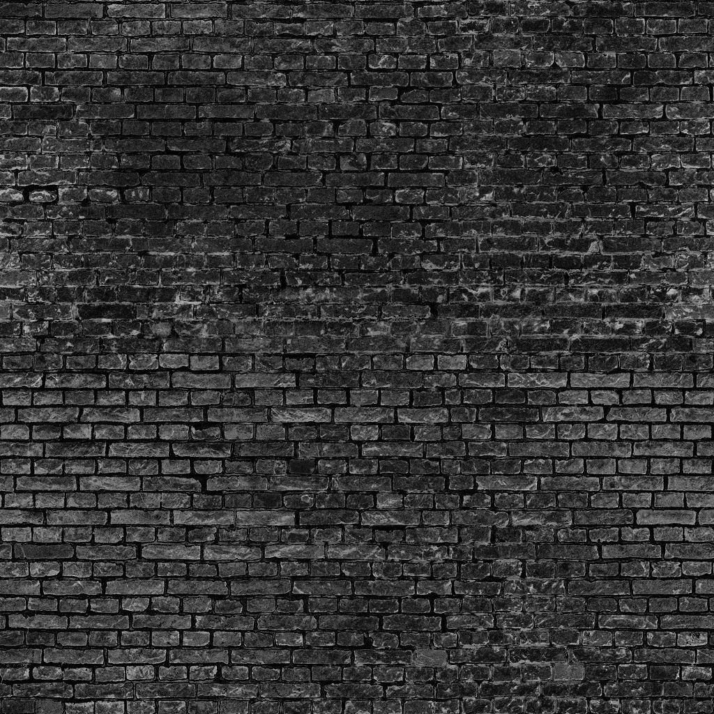
  (b) Change the texture of this cube object to one based on the file bricks_diffuse.png and turn off the flags for normal and specular textures.

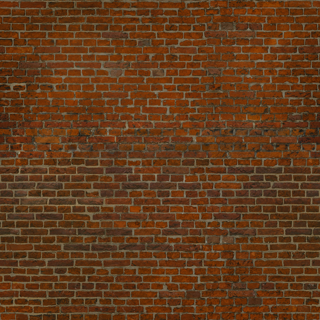
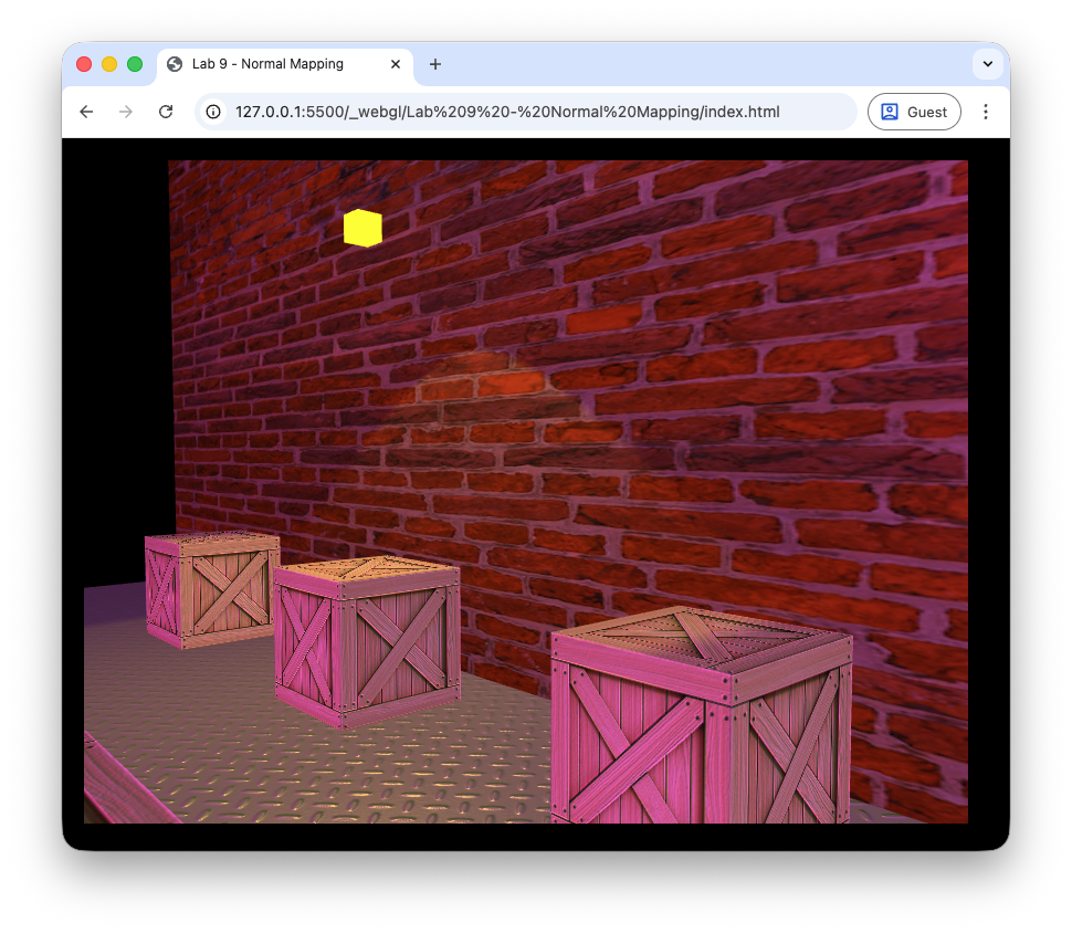
  (c) Add a normal map to the wall object based on the file bricks_normal.png.

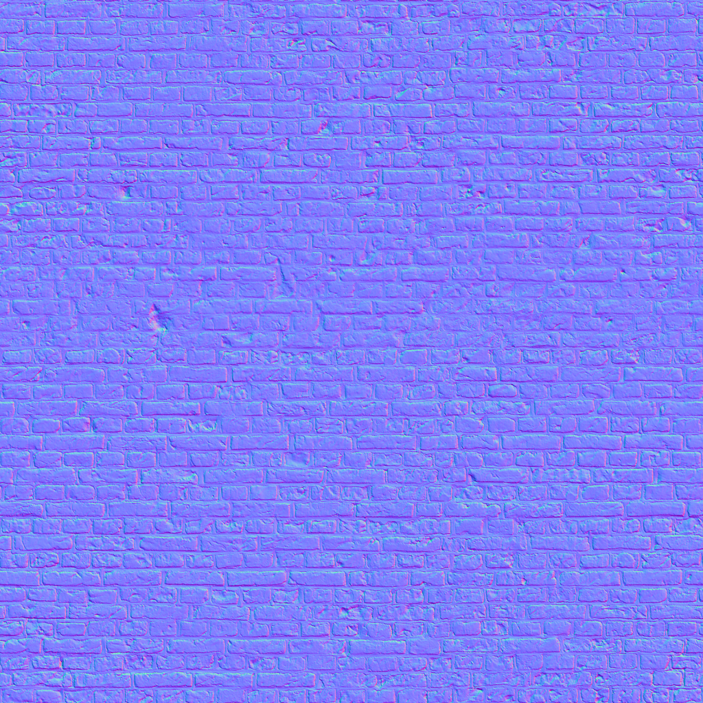
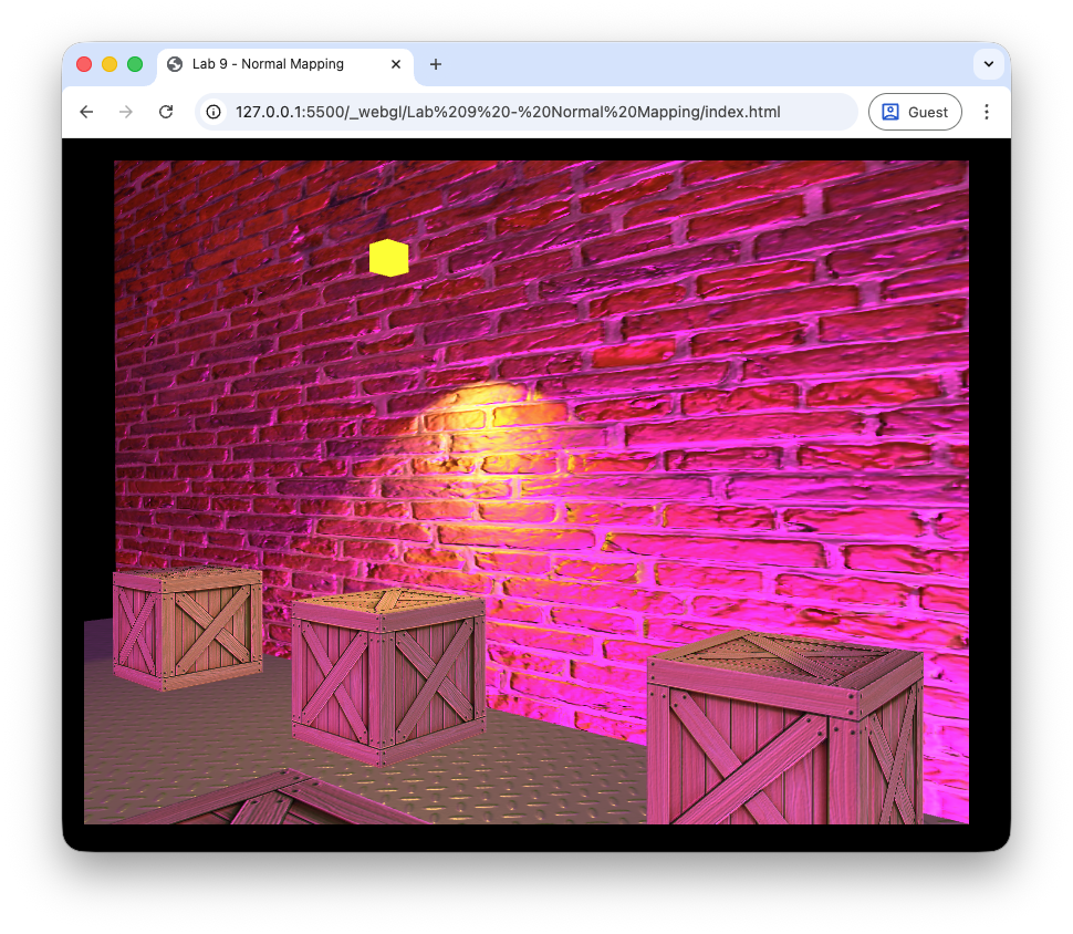
  (d) Add a specular map to the wall object based on the file bricks_specular.png.

---

Video walkthrough

The video below walks you through these lab materials.