Lab 7: Lighting

Lab 7: Lighting#

In this lab we will be looking at adding a basic lighting model to our application. Lighting modelling is in itself a huge topic within the field of computer graphics and modern games and movies can look very lifelike thanks to some very clever techniques. Here we will be applying one of the simplest lighting models, the Phong reflection model.

Task

Create a copy of your 06 Moving the Camera folder, rename it 07 Lighting, rename the file moving_the_camera.js to lighting.js and change index.html so that the page title is “Lab 7 - Lighting” it uses lighting.js.

To help demonstrate the effects of lighting on a scene we are going to need more objects, so we are going to draw more cubes.

Task

Change the definition of the cubes to the following.

// Define cube positions (5x5 grid of cubes)
const cubePositions = [];
for (let i = 0; i < 5; i++)  {
  for (let j = 0; j < 5; j++) {
    cubePositions.push([3 * i, 0, -3 * j]);
  }
}

// Define cubes
const numCubes = cubePositions.length;
const cubes = [];
for (let i = 0; i < numCubes; i++) {
  cubes.push({
    position  : cubePositions[i],
  });
}

Also, change the gl.clearColor() command in the initWebGL() function.

gl.clearColor(0.0, 0.0, 0.0, 1.0);

Here we have defined an array called cubes that contains JavaScript objects that define the positions of the centre coordinates of a set of cubes. Refresh your browser, and you can see that we have created a \(5 \times 5\) grid of cubes. We have also changed the background colour to black so that we can better see the lighting effects.

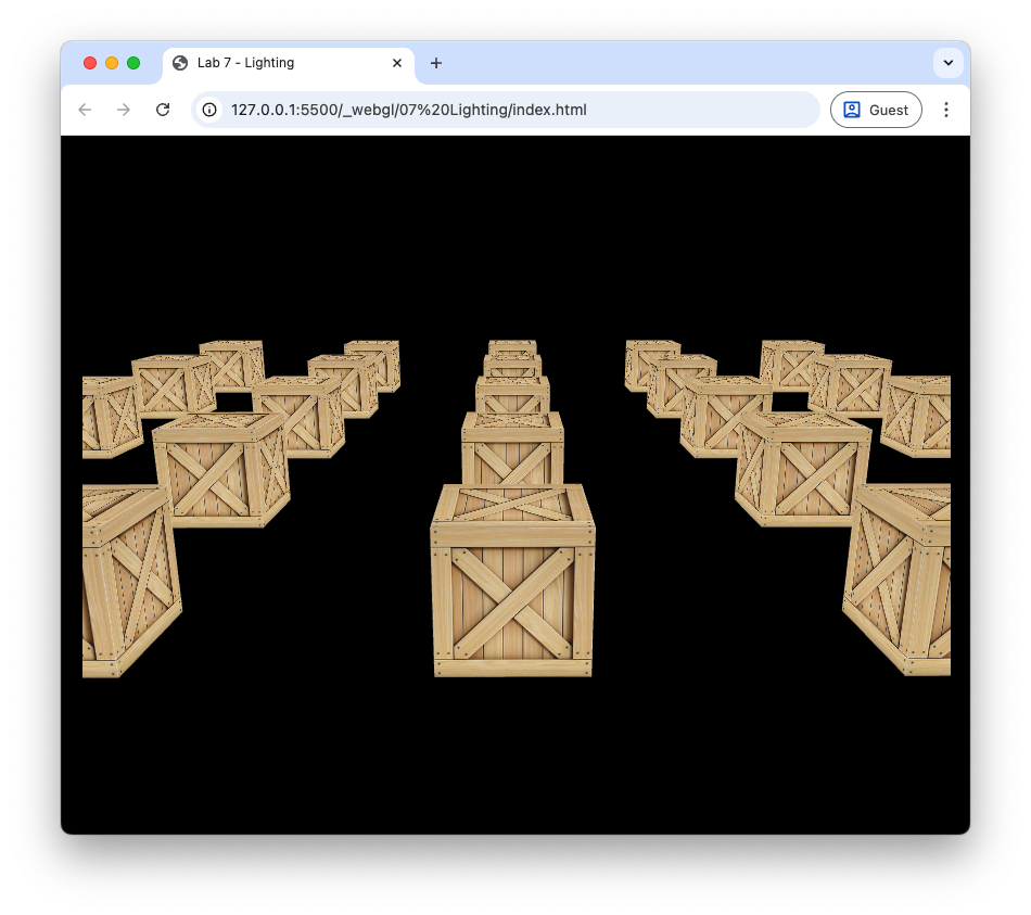
../_images/07_cubes.png — Fig. 65 Grid of 25 cubes.#

Phong’s lighting model#

Phong’s lighting model first described by Bui Tuong Phong is a local illumination model that simulates the interaction of light falling on surfaces. The brightness of a point on a surface is based on three components

ambient lighting – a simplified model of light that reflects off all objects in a scene
diffuse lighting – describes the direct illumination of a surface by a light source based on the angle between the light source direction and the normal vector to the surface
specular lighting – models the shiny highlights on a surface caused by a light source based on the angle between the light source direction, the normal vector and the view direction

The colour intensity of a fragment on the surface is calculated as a sum of these components, i.e.,

\[ \vec{colour} = \vec{ambient} + \vec{diffuse} + \vec{specular},\]

where theses are 3-element vectors of RGB colour values.

Ambient lighting#

Ambient lighting is light that is scatters off of all surfaces in a scene. To model this we make the simplifying assumption that all faces of the object is lit equally.Phong’s model for ambient lighting is

(22)#\[ \vec{ambient} = k_a \vec{O}_d \]

where \(k_a\) is known as the ambient lighting constant which takes on a value between 0 and 1 and \(\vec{O}_d\) is the object colour. \(k_a\) is a property of the object so we specify a value for this for each objects in our scene. The lighting calculations will be performed in the fragment shader and the fragment shader shown below applied ambient lighting to the scene.

#version 300 es
precision mediump float;

in vec3 vColour;
in vec2 vTexCoords;

out vec4 fragColour;

uniform sampler2D uTexture;

// Material coefficients
uniform float uKa;

void main() {

  // Object colour
  vec4 objectColour = texture(uTexture, vTexCoords);

  // Ambient
  vec3 ambient = uKa * objectColour.rgb;

  // Fragment colour
  fragColour = vec4(ambient, objectColour.a);
}

Note that here we are using swizzling to extract the RBG components of the object colour vector when calculating the ambient lighting where objectColour.rgb gives the first three components of the objectColour vector.

Task

Edit the fragment shader in the lighting.js file so that it looks like the fragment shader above.

We need now need to define \(k_a\) for the cube objects and send this to the shader.

Task

Edit the code used to define the cubes so that it looks like the following.

cubes.push({
  position  : cubePositions[i],
  ka        : 0.2,
});

And add the following code after the model matrix has been sent to the shader in the render() loop.

// Send object light properties to the shader
gl.uniform1f(gl.getUniformLocation(program, "uKa"), cubes[i].ka);

Refresh your web browser and you should see that the cubes are appear duller than compared to Fig. 65.

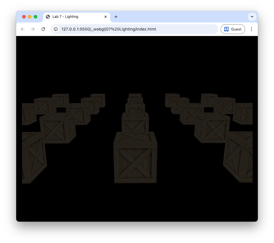
../_images/07_cubes_ambient_0.2.png — Fig. 66 Ambient lighting with \(k_a = 0.2\).#

Changing the value of \(k_a\) will make the colour of the cubes appear lighter or darker.

../_images/07_cubes_ambient_0.5.png — Fig. 67 \(k_a=0.5\)#

../_images/07_cubes_ambient_0.8.png — Fig. 68 \(k_a=0.8\)#

Diffuse lighting#

Diffuse lighting is where light is reflected off a rough surface. Consider Fig. 69 that shows parallel light rays hitting a surface where light is scattered in multiple directions.

../_images/07_diffuse_reflection.svg — Fig. 69 Light rays hitting a rough surface are scattered in all directions.#

To model diffuse lighting Phong’s model assumes that light is reflected equally in all directions (Fig. 70).

../_images/07_diffuse.svg — Fig. 70 Diffuse lighting scatters light equally in all directions.#

The amount of light that is reflected to the viewer is modelled using the angle \(\theta\) between the light vector \(\vec{L}\) which points from the fragment to the light source and the normal vector \(\vec{n}\) which points perpendicular to the surface. If \(\theta\) is small then the light source is directly in front of the surface so most of the light will be reflected to the viewer. Whereas if \(\theta\) is close to 90\(^\circ\) then the light source is nearly in line with the surface and little of the light will be reflected to the viewer. When \(\theta > 90^\circ\) the light source is behind the surface so no light is reflected to the viewer. We model this using \(\cos(\theta)\) since \(\cos(0^\circ) = 1\) and \(\cos(90^\circ)=0\). Diffuse lighting is calculated using

(23)#\[ \vec{diffuse} = k_d \vec{I}_p \vec{O}_d \cos(\theta) ,\]

where \(k_d\) is known as the diffuse lighting constant which takes a value between 0 and 1, and \(\vec{I}_p\) is the colour intensity of the point light source. Recall that the angle between two vectors is related by dot product so if the \(\vec{L}\) and \(\vec{n}\) vectors are unit vectors then \(\cos(\theta) = \vec{L} \cdot \vec{n}\). If \(\theta > 90^\circ\) then light source is behind the surface and no light should be reflected to the viewer. When \(\theta\) is between 90\(^\circ\) and 180\(^\circ\), \(\cos(\theta)\) is negative so we limit the value of \(\cos(\theta )\) to positive values

\[ \cos(\theta) = \max(\vec{L} \cdot \vec{n}, 0). \]

So the equation to calculate diffuse reflection is

\[ \vec{diffuse} = k_a \max(\vec{L} \cdot \vec{n}, 0) \vec{I}_p \vec{O}_d. \]

The world space fragment position is calculated by multiplying the vertex position by the model matrix, however the world space normal vector is calculated using the following transformation

\[ \begin{align*} \vec{n} = (Model^{-1})^\mathsf{T} \vec{n} \end{align*} \]

Recall that \(A^\mathsf{T}\) is the transpose and \(A^{-1}\) is the inverse of the matrix \(A\) such that \(A^{-1}A = I\). We use this transformation to ensure that the normal vector is perpendicular to the surface after the object vertices have been multiplied by the model matrix. You don’t need to know where this comes from but if you are interested, click on the dropdown link below.

Each vertex of our cube object needs to have an associated normal vector (Fig. 73). The normals for the front face will point in the positive \(z\) direction so \(\vec{n} = (0, 0, 1)\), the normals for the right face will point in the positive \(x\) direction so \(\vec{n} = (1, 0, 0)\), and similar for the other faces of the cube.

../_images/07_cube_normals.svg — Fig. 73 Each vertex of the cube has an associated normal vector.#

Task

Add the \(x\), \(y\) and \(z\) components of the normal vector to each cube vertex.

// Define cube vertices
  const vertices = new Float32Array([
    // x  y  z      r  g  b     u  v     nx  ny  nz                   + ------ +
    // front                                                         /|       /|
    -1, -1,  1,     0, 0, 0,    0, 0,    0,  0,  1,  //    y        / |      / |
     1, -1,  1,     0, 0, 0,    1, 0,    0,  0,  1,  //    |       + ------ +  |
     1,  1,  1,     0, 0, 0,    1, 1,    0,  0,  1,  //    +-- x   |  + ----|- +
    -1, -1,  1,     0, 0, 0,    0, 0,    0,  0,  1,  //   /        | /      | /
     1,  1,  1,     0, 0, 0,    1, 1,    0,  0,  1,  //  z         |/       |/
    -1,  1,  1,     0, 0, 0,    0, 1,    0,  0,  1,  //            + ------ +
    // right
     1, -1,  1,     0, 0, 0,    0, 0,    1,  0,  0,
     1, -1, -1,     0, 0, 0,    1, 0,    1,  0,  0,
     1,  1, -1,     0, 0, 0,    1, 1,    1,  0,  0,
     1, -1,  1,     0, 0, 0,    0, 0,    1,  0,  0,
     1,  1, -1,     0, 0, 0,    1, 1,    1,  0,  0,
     1,  1,  1,     0, 0, 0,    0, 1,    1,  0,  0,
    // etc.

In the createVao() method in the webGLUtils.js file, change the stride to 11 since we now have an additional 3 elements per vertex.

const stride = 11 * Float32Array.BYTES_PER_ELEMENT;

And in the same function tell WebGL how to read the normal vectors

// Normal vectors
offset = 8 * Float32Array.BYTES_PER_ELEMENT;
const normalLocation = gl.getAttribLocation(program, "aNormal");
gl.enableVertexAttribArray(normalLocation);
gl.vertexAttribPointer(normalLocation, 3, gl.FLOAT, false, stride, offset);

Now change the vertex shader to accept the normals as an input attribute and an output.

in vec3 aNormal;

out vec3 vNormal;

And in the main() function calculate the world space normal preserving orthogonality with the face.

// Output world space normal vectors
vNormal = normalize(mat3(transpose(inverse(uModel))) * aNormal);

Now change the fragment shader to accept the normal as an input

in vec3 aNormal;

Lastly, set the fragment colour to the normal vector.

// Fragment colour
fragColour = vec4(vNormal, objectColour.a);

Phew! If everything has gone ok when you refresh your web browser you should see the three sides of the cubes are rendered in varying shades of red, green and blue. What we have done here is used the world space normal vector as the fragment colour as a check to see if everything is working as expected. Move the camera around, and you will notice that the side of the closest cube facing to the right is red because its normal vector is \((1, 0, 0)\) so in RGB this is pure red. The side facing up is green because its normal vector is \((0, 1, 0)\) and the side facing towards us is blue because its normal vector is \((0, 0, 1)\) as shown in Fig. 74. The sides of the cubes that have been rotated are varying shades of red, green and blue based on the direction their normals are pointing.

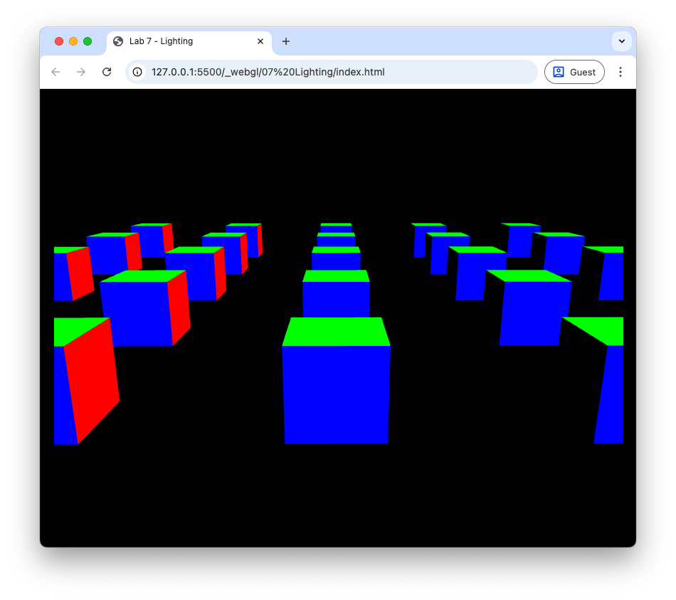
../_images/07_cubes_normals.png — Fig. 74 The colours of the cube faces based on the normal vectors.#

Now we just need to define diffuse coefficient for the cubes, the position and colour of our light source and send them to the shaders using uniforms.

Task

Edit the commands used to define the cubes to include the diffuse coefficient \(k_d = 0.7\).

kd        : 0.7,

Now define a JavaScript object for the light source properties just after where we have defined the cube positions and lighting coefficients.

// Define light source properties
const light = {
  position  : [2, 2, 2],
  colour    : [1, 1, 1],
}

Send the light position and colour vectors to the shaders after we have done this for the view and projection matrices.

// Send light source properties to the shader
gl.uniform3fv(gl.getUniformLocation(program, "uLightPosition"), light.position);
gl.uniform3fv(gl.getUniformLocation(program, "uLightColour"), light.colour);

And send the diffuse coefficient to the shader where we did this for the ambient coefficient.

gl.uniform1f(gl.getUniformLocation(program, "uKd"), cubes[i].kd);

Now we have sent all the information required for diffuse lighting to the shader we now just need to edit the shaders.

Task

Add output declarations to the vertex shader so that it outputs the world space vertex coordinates.

out vec3 vPosition;

And add the following code after we output the world space normal vectors.

// Output world space vertex position
vPosition = vec3(uModel * vec4(aPosition, 1.0));

Add input declarations to the fragment shader to take in the world space fragment coordinates.

in vec3 vPosition;

Add uniform declarations for the light position and colour and the diffuse coefficient.

uniform vec3 uLightPosition;
uniform vec3 uLightColour;

uniform float uKd;

Finally, add code to calculate diffuse lighting.

// Diffuse
vec3 N = normalize(vNormal);
vec3 L = normalize(uLightPosition - vPosition);
vec3 diffuse = uKd * max(dot(N, L), 0.0) * uLightColour * objectColour.rgb;

// Fragment colour
fragColour = vec4(diffuse, objectColour.a);

It is useful to render an object for the light source so that we can see where it is positioned in the scene. To do this we will use a cube object scaled down to a small size and rendered using a simple shader that colours the cube with the light source colour.

Task

Define the vertex and fragment shaders for the light source cube at the top of the lighting.js file.

// Define vertex and fragment shaders for the light source
const lightVertexShader =
`#version 300 es
precision mediump float;

in vec3 aPosition;

uniform mat4 uModel;
uniform mat4 uView;
uniform mat4 uProjection;

void main() {
  gl_Position = uProjection * uView * uModel * vec4(aPosition, 1.0);
}`;

const lightFragmentShader =
`#version 300 es
precision mediump float;

out vec4 fragColour;

uniform vec3 uLightColour;

void main() {
  fragColour = vec4(uLightColour, 1.0);
}`;

Compile and link the light source shaders after the main shader program has been created.

const lightProgram = createProgram(gl, lightVertexShader, lightFragmentShader);

In the render() loop, after rendering the cubes, add the following code to render the light source cube.

// Render light source
gl.useProgram(lightProgram);

// Calculate model matrix for light source
const translate = new Mat4().translate(...light.position);
const scale     = new Mat4().scale(0.1, 0.1, 0.1);
const model     = translate.multiply(scale);
gl.uniformMatrix4fv(gl.getUniformLocation(lightProgram, "uModel"), false, model.m);
gl.uniformMatrix4fv(gl.getUniformLocation(lightProgram, "uView"), false, view.m);
gl.uniformMatrix4fv(gl.getUniformLocation(lightProgram, "uProjection"), false, projection.m);

// Send light colour to the shader
gl.uniform3fv(gl.getUniformLocation(lightProgram, "uLightColour"), light.colour);

// Draw light source cube
gl.bindVertexArray(vao);
gl.drawElements(gl.TRIANGLES, 36, gl.UNSIGNED_SHORT, 0);

Refresh your web browser, and you should see the effect of diffuse lighting on the cubes (Fig. 75). Here we can see the light source cube in white and the faces of the cubes that are facing towards the light source are brighter than those facing away.

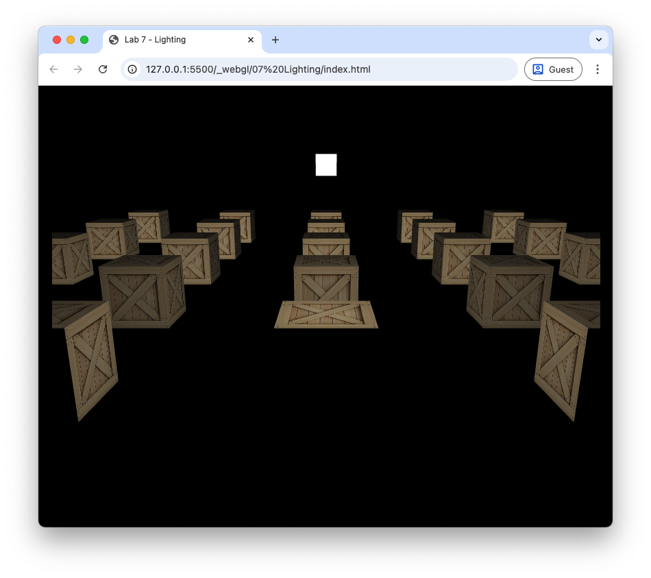
../_images/07_cubes_diffuse.png — Fig. 75 Diffuse lighting: \(k_d = 0.7\).#

If you move the camera around, you will see that the faces of the cubes that are facing away from the light source are black since we have not factored in ambient lighting, so let’s include that now.

Task

Change the fragment shader so that the fragment colour is the sum of the ambient and diffuse lighting.

fragColour = vec4(ambient + diffuse, objectColour.a);

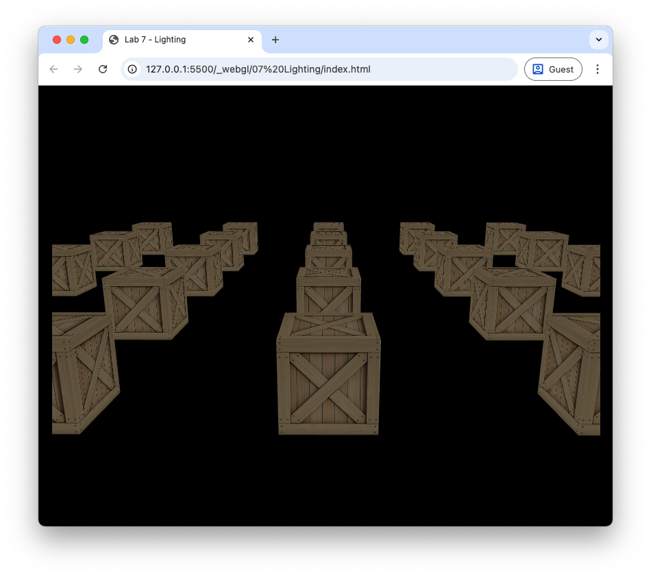
Refresh your web browser, and you should see the cubes rendered with both ambient and diffuse lighting (Fig. 76).

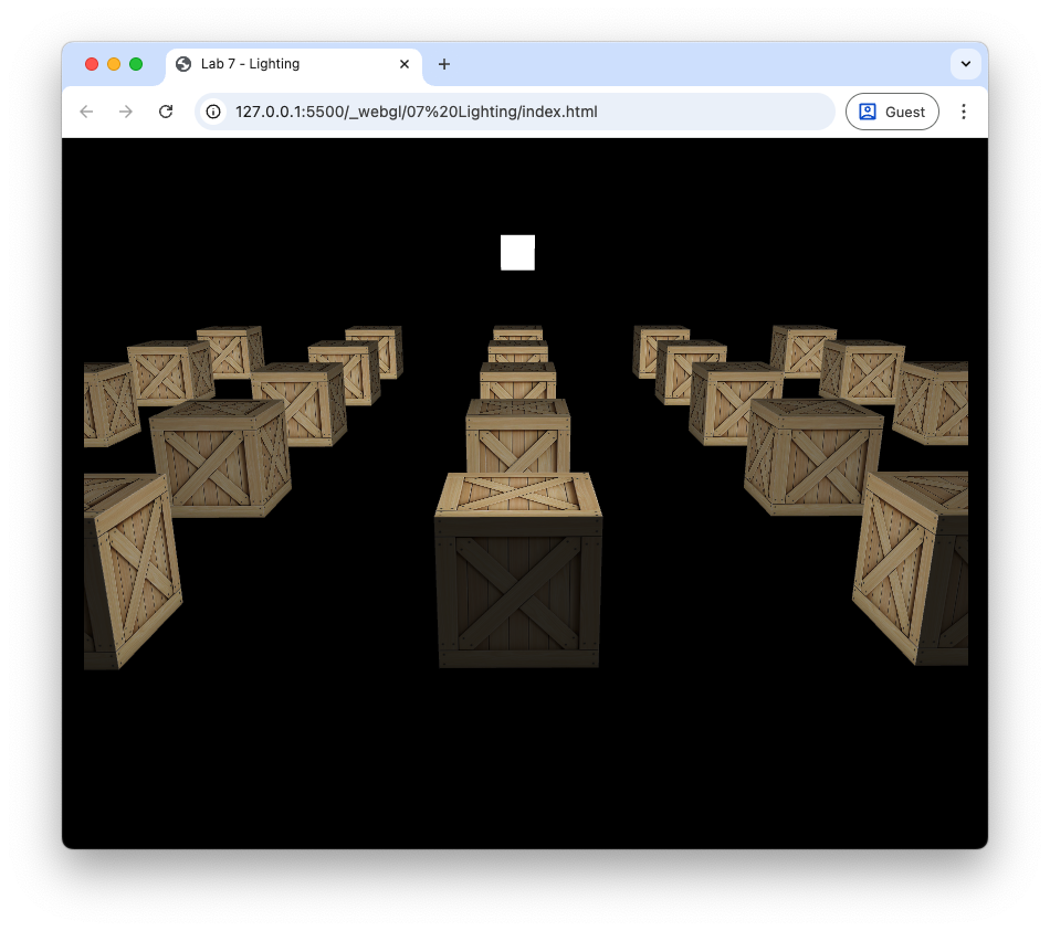
../_images/07_cubes_ambient_diffuse.png — Fig. 76 Ambient and diffuse lighting: \(k_a = 0.2\), \(k_d = 0.7\).#

Specular lighting#

Consider Fig. 77 that shows parallel light rays hitting a smooth surface where the reflected rays will point mostly in the same direction (think of a mirrored surface).

../_images/07_specular_reflection.svg — Fig. 77 Light rays hitting a smooth surface are reflected in the same direction.#

Specular lighting depends upon the position of the light source and the fragment in the world space. Consider Fig. 78 that shows a surface with a normal vector \(\vec{n}\), a vector \(\vec{L}\) pointing from the surface to a light source and a vector \(\vec{R}\) pointing in the direction of reflected light off the surface. The angle between \(\vec{L}\) and \(\vec{n}\), \(\theta\) which is known as the incidence angle, and the angle between \(\vec{R}\) and \(\vec{n}\) are the same.

../_images/07_reflection.svg — Fig. 78 The light vector is reflected about the normal vector.#

If \(\vec{n}\) and \(\vec{L}\) are unit vectors then the \(\vec{R}\) vector is calculated using

\[ \begin{align*} \vec{R} = - \vec{L} + 2 (\vec{L} \cdot \vec{n}) \vec{n} \end{align*} \]

If you are interested in the derivation of this formula, click on the dropdown below.

For a perfectly smooth surface the reflected ray will point in the direction of the \(\vec{R}\) vector so in order to see the light the viewer would need to be positioned in the direction of the \(\vec{R}\) vector. The viewing vector \(\vec{V}\) is the vector that points from the surface to the viewer (camera). Since most surfaces are not perfectly smooth we add a bit of scattering to the model the amount of specular lighting seen by the viewer. This is determined by the angle \(\phi\) between the \(\vec{R}\) vector and the \(\vec{V}\) vector. The closer the viewing vector is to the reflection vector, the smaller the value of \(\phi\) will be and the more of the light will be reflected towards the camera.

../_images/07_specular.svg — Fig. 81 Specular lighting scatters light mainly towards the reflection vector.#

Phong modelled the scattering of the reflected light rays using \(\cos(\phi)\) raised to a power

\[\vec{specular} = k_s \vec{I}_p \cos(\phi)^{\alpha},\]

where \(k_s\) is the specular lighting coefficient similar to its ambient and diffuse counterparts and \(\alpha\) is the specular exponent that determines the shininess of the object. If \(\vec{R}\) and \(\vec{V}\) are unit vectors, then \(\cos(\phi)\) can be calculated using \( \cos(\phi) = \max(\vec{V} \cdot \vec{R}, 0)^{\alpha}\), so the specular reflection equation is

(24)#\[ \vec{specular} = k_s \max(\vec{V} \cdot \vec{R}, 0)^\alpha \vec{I}_p.\]

Task

Add the specular coefficient and exponent to the cube objects where we did the same for the ambient and diffuse coefficients.

ks        : 1.0,
shininess : 32,

And send them to the shader where we did this for the ambient and diffuse coefficients.

gl.uniform1f(gl.getUniformLocation(program, "uKs"), cubes[i].ks);
gl.uniform1f(gl.getUniformLocation(program, "uShininess"), cubes[i].shininess);

Send the camera position to the shader after we sent the light position and colour.

// Send camera position to the shader
gl.uniform3fv(gl.getUniformLocation(program, "uCameraPosition"), camera.eye.array);

And send the specular coefficient and exponent to the shader where we did this for the ambient and diffuse coefficients.

gl.uniform1f(gl.getUniformLocation(program, "uKs"), cubes[i].ks);
gl.uniform1f(gl.getUniformLocation(program, "uShininess"), cubes[i].shininess);

Now in the fragment shader, add uniforms for the camera position, specular coefficient and exponent.

uniform vec3 uCameraPosition;

uniform float uKs;
uniform float uShininess;

And add code to calculate the specular lighting in the main() function.

// Specular
vec3 V = normalize(uCameraPosition - vPosition);
vec3 R = reflect(-L, N);
vec3 specular = uKs * pow(max(dot(R, V), 0.0), uShininess) * uLightColour;

// Fragment colour
fragColour = vec4(specular, objectColour.a);

Refresh your web browser and your scene should be very dark. Move the camera so that the cubes are between the camera and the light source and you should start to see the specular highlights where light is being reflected off the cube Fig. 82.

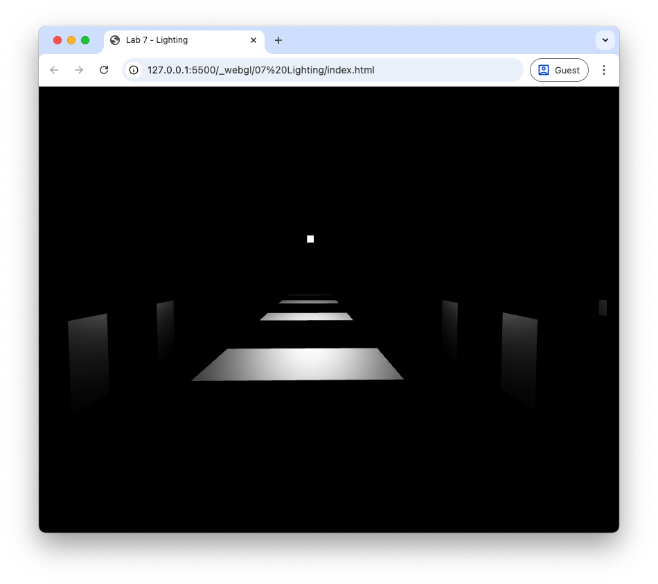
../_images/07_cubes_specular.png — Fig. 82 Specular lighting: \(k_s = 1.0\), \(\alpha = 20\).#

Let’s add ambient and diffuse lighting to the specular lighting to complete the Phong reflection model.

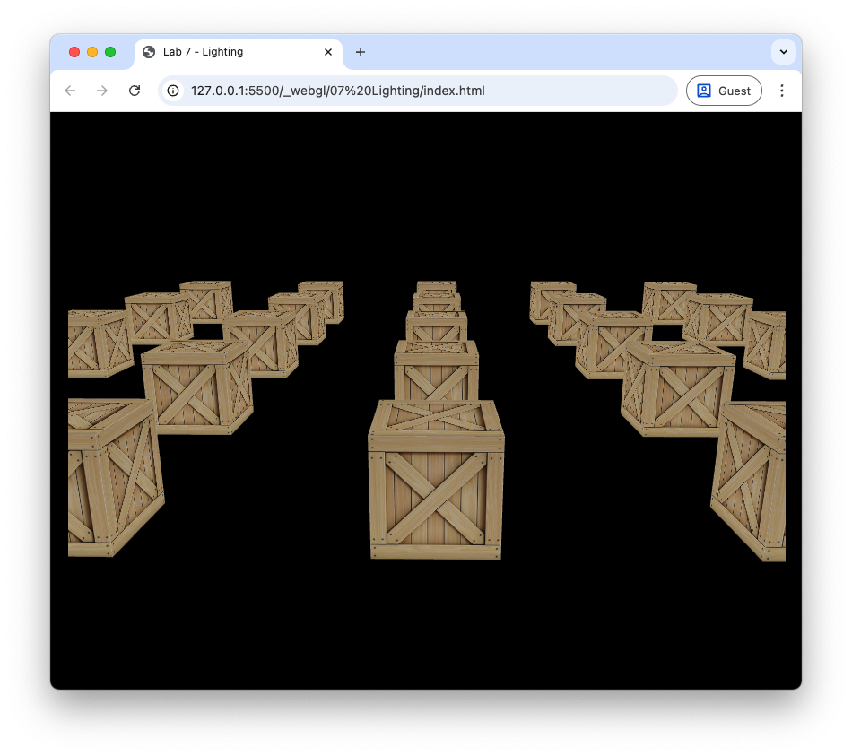
Task

Change the fragment shader so that the fragment colour is the sum of the ambient, diffuse and specular lighting.

fragColour = vec4(ambient + diffuse + specular, objectColour.a);

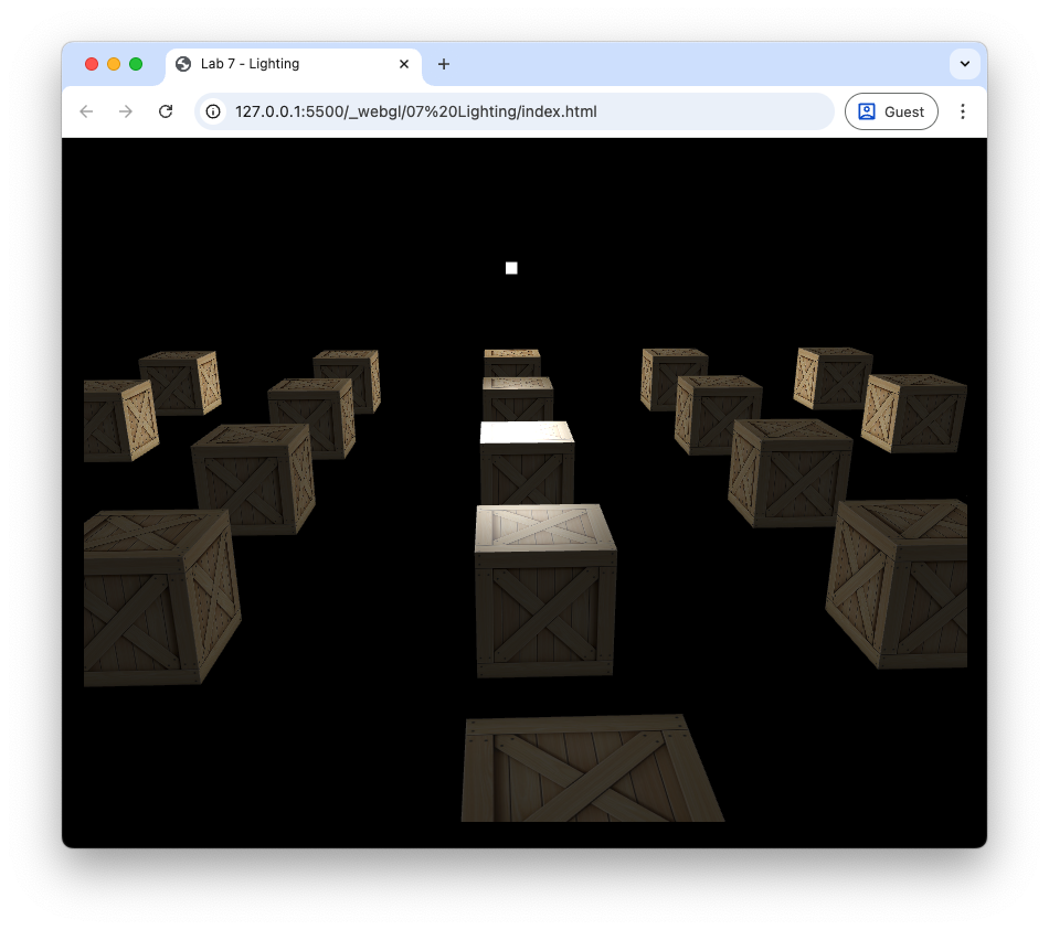
../_images/07_cubes_phong.png — Fig. 83 Ambient, diffuse and specular lighting: \(k_a = 0.2\), \(k_d = 0.7\), \(k_s = 1.0\), \(\alpha = 20\).#

Attenuation#

Attenuation is the gradual decrease in light intensity as the distance between the light source and a surface increases. We can use attenuation to model light from low intensity light source, for example, a candle or torch which will only illuminate an area close to the source. Theoretically attenuation should follow the inverse square law where the light intensity is inversely proportional to the square of the distance between the light source and the surface. However, in practice this tends to result in a scene that is too dark so we calculate attenuation using an inverse quadratic function

\[ attenuation = \frac{1}{constant + linear \cdot d + quadratic \cdot d^2}, \]

where \(d\) is the distance between the light source and the fragment and \(constant\), \(linear\) and \(quadratic\) are coefficients that determine how quickly the light intensity decreases. The graph in Fig. 84 shows a typical attenuation profile where the light intensity rapidly decreases when the distance is small levelling off as the distance gets larger.

../_images/07_attenuation.svg — Fig. 84 Attenuation can be modelled by an inverse quadratic function.#

Task

Add the following attenuation coefficients to the light source.

constant  : 1.0,
linear    : 0.1,
quadratic : 0.02,

And send them to the shader where we did this for the light source position and colour.

gl.uniform1f(gl.getUniformLocation(program, "uConstant"), light.constant);
gl.uniform1f(gl.getUniformLocation(program, "uLinear"), light.linear);
gl.uniform1f(gl.getUniformLocation(program, "uQuadratic"), light.quadratic);

Add the uniforms to the fragment shader.

// Attenuation parameters
uniform float uConstant;
uniform float uLinear;
uniform float uQuadratic;

Then calculate and apply attenuation to the fragment colour.

// Attenuation
float dist = length(uLightPosition - vPosition);
float attenuation = 1.0 / (uConstant + uLinear * dist + uQuadratic * dist * dist);

// Fragment colour
fragColour = vec4(attenuation * (ambient + diffuse + specular), objectColour.a);

These values used the attenuation ceofficients here depend on the type of light source being modelled. In this case we have a weak light source to demonstrate the loss of light intensity over space but for stronger light sources you may wish to experiment with these values. Refresh your web browser and you should see that the cubes further away from the light source are darker as shown in Fig. 85.

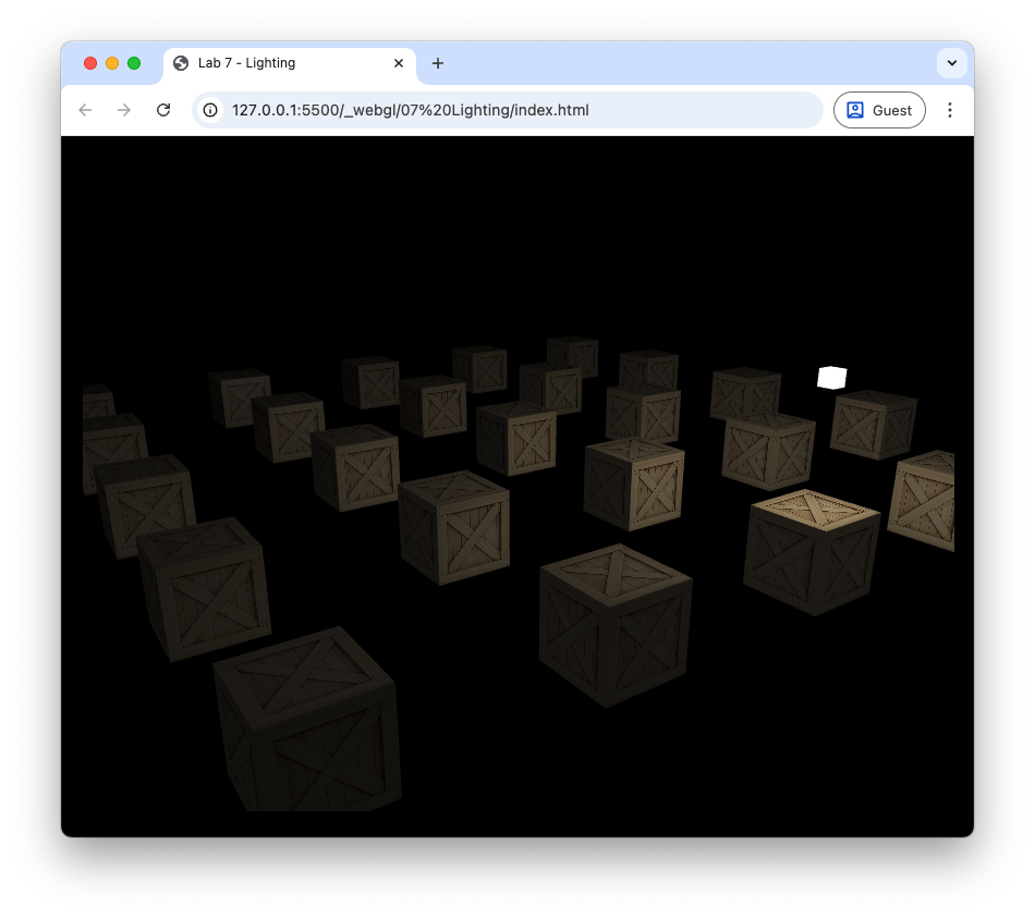
../_images/07_cubes_attenuation.png — Fig. 85 Applying attenuation means that the objects further away from light source appear darker.#

Multiple light sources#

To add more light sources to a scene is simply a matter of calculating the ambient, diffuse and specular reflection for each additional light source and then adding them to the fragment colour. We have seen for a single light source we have to define the light source colours, the position of the light source in the world space and the three attenuation constants. Given that we would like to do this for multiple light sources we need data structure for each light source.

A data structure in GLSL is defined as follows:

struct Light {
  int type;
  vec3 position;
  vec3 colour;
  float constant;
  float linear;
  float quadratic;
};

This defines a Light structure with attributes for the light source type, position, colour and attenuation constants. The type attribute will be used later to specify different types of light sources. Before we add additional light sources we are going to rewrite our fragment shader to use a data structure.

#version 300 es
precision mediump float;

in vec3 vColour;
in vec2 vTexCoords;
in vec3 vNormal;
in vec3 vPosition;

out vec4 fragColour;

uniform sampler2D uTexture;
uniform vec3 uCameraPosition;

// Material coefficients
uniform float uKa;
uniform float uKd;
uniform float uKs;
uniform float uShininess;

// Light struct
struct Light {
  int type;
  vec3 position;
  vec3 colour;
  float constant;
  float linear;
  float quadratic;
};

// Number of lights
uniform int uNumLights;

// Array of lights
uniform Light uLights[16];

// Function to calculate diffuse and specular reflection
vec3 computeLight(Light light, vec3 N, vec3 V, vec3 objectColour){
 
  // Light vector
  vec3 L = normalize(light.position - vPosition);

  // Reflection vector
  vec3 R = reflect(-L, N);

  // Attenuation
  float dist = length(light.position - vPosition);
  float attenuation = 1.0 / (light.constant + light.linear * dist + light.quadratic * dist * dist);

  // Ambient reflection
  vec3 ambient = uKa * objectColour;

  // Diffuse
  vec3 diffuse = uKd * max(dot(N, L), 0.0) * light.colour * objectColour;

  // Specular
  vec3 specular = uKs * pow(max(dot(R, V), 0.0), uShininess) * light.colour;

  // Output fragment colour
  return attenuation * (ambient + diffuse + specular);
}

// Main function
void main() {

  // Object colour
  vec4 objectColour = texture(uTexture, vTexCoords);

  // Lighting vectors
  vec3 N = normalize(vNormal);
  vec3 V = normalize(uCameraPosition - vPosition);

  // Calculate lighting for each light source
  vec3 result;
  for (int i = 0; i < 16; i++) {
    if (i >= uNumLights) break;
    result += computeLight(uLights[i], N, V, objectColour.rgb);
  }

  // Fragment colour
  fragColour = vec4(result, objectColour.a);
}

This fragment shader is a little more complex than before but the main changes are:

A Light data structure is defined with attributes for the light source type, position, colour and attenuation constants.
An array of Light structures called uLights is defined to hold up to 16 light sources.
A uniform integer uNumLights is defined to specify the number of active light sources.
A function computeLight() is defined to calculate the diffuse and specular reflection for a given light source.
In the main() function a for loop iterates over the active light sources and calls the computeLight() function for each light source to add its contribution to the fragment colour.

Since this fragment shader not uses an array of light source we need to update the more_lights.js file to define multiple light sources using the Light data structure and send them to the shader.

Task

Edit the fragment shader in the more_lights.js file to use the new fragment shader above.

Define an array containing the properties of two light sources.

// Create vector of light sources
const lightSources = [ 
  {
    type        : 1,
    position    : [6, 2, 0],
    colour      : [1, 1, 1],
    direction   : [0, -1, -2],
    constant    : 1.0,
    linear      : 0.1,
    quadratic   : 0.02,
  },
  {
    type        : 1,
    position    : [9, 2, -9],
    direction   : [0, 0, 0],
    colour      : [1, 1, 0],
    constant    : 1.0,
    linear      : 0.1,
    quadratic   : 0.02,
  },
];

Edit the code where the light source properties are sent to the shader to loop over the lightSources array and send each light source’s properties to the shader.

// Send light source properties to the shader
gl.uniform1i(gl.getUniformLocation(program, "uNumLights"), numLights);
for (let i = 0; i < numLights; i++) {
  gl.uniform1i(gl.getUniformLocation(program, `uLights[${i}].type`), lightSources[i].type);
  gl.uniform3fv(gl.getUniformLocation(program, `uLights[${i}].position`), lightSources[i].position);
  gl.uniform3fv(gl.getUniformLocation(program, `uLights[${i}].colour`), lightSources[i].colour);  
  gl.uniform1f(gl.getUniformLocation(program, `uLights[${i}].constant`), lightSources[i].constant);
  gl.uniform1f(gl.getUniformLocation(program, `uLights[${i}].linear`), lightSources[i].linear);
  gl.uniform1f(gl.getUniformLocation(program, `uLights[${i}].quadratic`), lightSources[i].quadratic);
}

And edit the code where the light sources are drawn to loop over the number of light sources.

// Render light sources
gl.useProgram(lightProgram);

for (let i = 0; i < numLights; i++) {
  // Calculate model matrix for light source
  const translate = new Mat4().translate(...lightSources[i].position);
  const scale     = new Mat4().scale(0.1, 0.1, 0.1);
  const model     = translate.multiply(scale);
  gl.uniformMatrix4fv(gl.getUniformLocation(lightProgram, "uModel"), false, model.m);
  gl.uniformMatrix4fv(gl.getUniformLocation(lightProgram, "uView"), false, view.m);
  gl.uniformMatrix4fv(gl.getUniformLocation(lightProgram, "uProjection"), false, projection.m);

  // Send light colour to the shader
  gl.uniform3fv(gl.getUniformLocation(lightProgram, "uLightColour"), lightSources[i].colour);

  // Draw light source cube
  gl.bindVertexArray(vao);
  gl.drawElements(gl.TRIANGLES, 36, gl.UNSIGNED_SHORT, 0);
}

Here we have defined two light sources, with an additional yellow light source positioned further back in the scene. The code to send the light source properties to the shader and to draw the light sources has been updated to loop over the number of light sources defined in the lightSources array. Refresh your web browser, and you should see the following. Move the camera around the scene to see the effects of the light sources on the cubes.

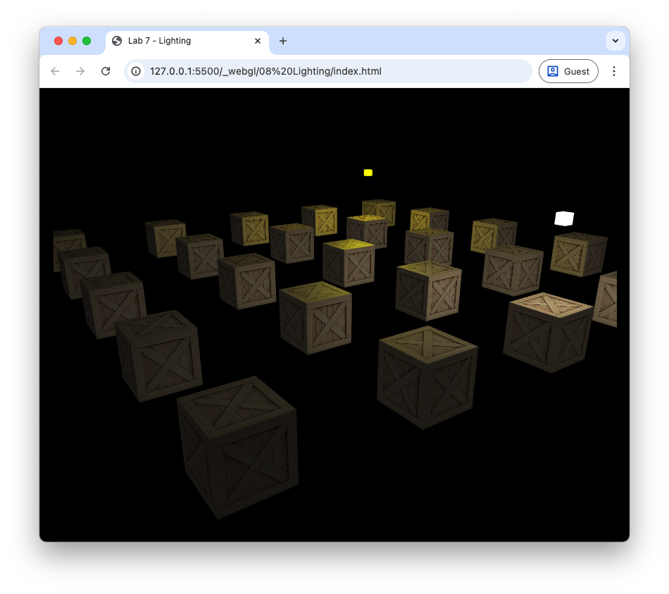
../_images/07_cubes_multiple_lights.png — Fig. 86 The cubes lit from two light sources.#

Spotlights#

Our light sources we have in our scene emit light in all directions. A spotlight is a light source that emits light along a specific direction so that only those objects that are within some distance of this vector are illuminated. These are useful for modelling light sources such as flashlights, streetlights, car headlights etc.

Consider Fig. 87 that shows a spotlight emitting light in the direction given by the \(\vec{D}\) vector. The \(\vec{L}\) vector points from the light source position to the position of the fragment and the spread of the spotlight is determined by the cutoff angle. If the angle \(\theta\) between \(\vec{L}\) and \(\vec{D}\) is less than the cutoff angle then the fragment is illuminated by the spotlight.

The angle between \(\vec{L}\) and \(\vec{D}\) is related to the dot product of the two vectors by

\[ \cos(\theta) = \vec{L} \cdot \vec{D}. \]

So to determine if a fragment is illuminated by the spotlight we can calculate \(\cos(\theta)\) and compare it to \(\cos(\textsf{cutoff})\). If \(\cos(\theta) < \cos(\textsf{cutoff})\) then \(\theta > \textsf{cutoff}\) and the fragment is not illuminated.

Task

Add attributes for the light direction vector and the value of \(\cos(\textsf{cutoff})\) to the Light data structure in the fragment shader.

vec3 direction;
float cutoff;

In the computeLight() function, add the following code to turn off the light contribution if the fragment is outside the spotlight cone.

// Spotlight
float spotLight = 1.0;
if (light.type == 2) {
  vec3 D = normalize(light.direction);
  float theta = dot(-L, D);
  spotLight = 0.0;
  if (theta > light.cutoff) {
    spotLight = 1.0;
  }
}

And apply the spotlight to the fragment colour calculation.

// Output fragment colour
return spotlight * attenuation * (ambient + diffuse + specular);

In the main() function, add the light direction and cutoff attributes to both light sources. In the first light source add the following and comment out the code definining the second light source.

type      : 2,
direction : [0, -1, -1],
cutoff    : Math.cos(40 * Math.PI / 180),

Finally, send the additional light source properties to the shader by adding the following code where the other light source properties are sent.

gl.uniform3fv(gl.getUniformLocation(program, `uLights[${i}].direction`), lightSources[i].direction);      
gl.uniform1f(gl.getUniformLocation(program, `uLights[${i}].cutoff`), lightSources[i].cutoff);

Here we have changed the first light source to be a spotlight that is pointing downwards and slightly towards the back of the scene. The cutoff angle is set to \(30^\circ\) by calculating \(\cos(30^\circ)\). The second light source has been switched off by commenting out the code that defines it. Refresh your web browser and you should see the following.

../_images/07_cubes_spotlight_harsh.png — Fig. 88 Cubes lit using a spotlight.#

Use the keyboard and mouse to move the camera around the cubes and see the effect of the spotlight. You may notice that there is an abrupt cutoff between the region illuminated by the spotlight and the region in darkness. In the real world this doesn’t usually happen as light on this edge gets softened by various effects.

We can model this softening by gradually reducing the intensity of the light as we approach the cutoff angle. Introducing a new inner cutoff angle that is slightly less than the cutoff angle then we can have full intensity for angles less than the inner cutoff angle and zero intensity for angles greater than the cutoff angle. Between these two angles we can gradually reduce the intensity from 1 to 0.

../_images/07_soft_edge.svg — Fig. 89 Intensity value over a range of \(\theta\).#

Task

Add an attribute for the inner cutoff angle to the Light data structure in the fragment shader.

float innerCutoff;

And in the computeLight() function, replace the spotlight code with the following code to soften the edges of the spotlight.

// Spotlight
float spotLight = 1.0;
if (light.type == 2) {
  vec3 D = normalize(light.direction);
  float theta = dot(-L, D);
  float epsilon = light.cutoff - light.innerCutoff;
  spotLight = clamp((light.cutoff - theta) / epsilon, 0.0, 1.0);
}

Now add the attibute to the light source definitions in the more_lights.js file.

innerCutoff : Math.cos(30 * Math.PI / 180),

And send the additional light source property to the shader by adding the following code where the other light source properties are sent.

gl.uniform1f(gl.getUniformLocation(program, `uLights[${i}].innerCutoff`), lightSources[i].innerCutoff);

Here we have defined an inner cutoff angle of \(25^\circ\) which is slightly less than the cutoff angle of \(30^\circ\). Refresh your web browser and you should see the following.

../_images/07_cubes_spotlight_soft.png — Fig. 90 The edges of the spotlight have been softened.#

Directional light#

The final light source type we will look at is directional light. When a light source is far away the light rays are very close to being parallel. It does not matter where the object is in the view space as all objects are lit from the same direction.

The lighting calculations are the same as for the other light sources seen above with the exception that we do not need the light source position and we do not apply the attenuation. The light vector \(\vec{L}\) is simply the light direction vector negated.

Task

Add the following after we have calculated the light vector in the computeLight() function in the fragment shader.

if (light.type == 3) {
  L = normalize(-light.direction);
}

And replace the code used to calculate the attenuation with the following.

// Attenuation
float attenuation = 1.0;
if (light.type != 3) {
  float dist = length(light.position - vPosition);
  attenuation = 1.0 / (light.constant + light.linear * dist + light.quadratic * dist * dist);
}

In the more_lights.js file, add an additional light source to the light sources array.

{
  type        : 3,
  position    : [0, 0, 0],
  direction   : [2, -1, -1],
  colour      : [1, 0, 1],
  constant    : 1.0,
  linear      : 0.1,
  quadratic   : 0.02,
  cutoff      : 0,
  innerCutoff : 0,
},

Finally, uncomment the code defining the other two light sources.

Here we have defined a directional light source with the direction vector \((2, -1, -1)\) which will produce light rays coming down from the top right as we look down the \(z\)-axis. The light source colour has been set to magenta using the RGB values \((1, 0, 1)\). Refresh your web browser and you should see the following.

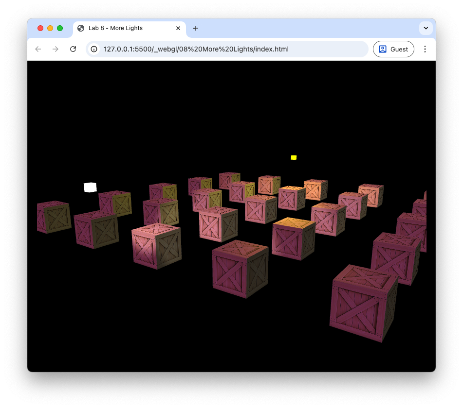
../_images/07_cubes_directional_light.png — Fig. 92 Cubes lit using a point light, spotlight and directional light.#

Exercises#

Experiment with the positions, colours and material properties of the various light sources to see what effects they have.
Use a spotlight to model a flashlight controlled by the user such that the light is positioned at \(\vec{eye}\), is pointing in the same direction as \(\vec{front}\) and has a spread angle of \(\phi = 15^\circ\). Turn off all other light sources for extra spookiness.
Change the colour of the second point light source to magenta and rotate its position in a circle centred at (0,0,-5) with radius 5. Turn off the spotlight and directional light. Hint: the coordinates of points on a circle can be calculated using \((x, y, z) = (c_x, c_y, c_z) + r (\cos(t), 0, \sin(t))\) where \(r\) is the radius \(t\) is some parameter (e.g., time).
Add the ability to turn the lights off and on using keyboard input.

Video walkthrough#

The video below walks you through these lab materials.

Lab 7: Lighting

Contents

Lab 7: Lighting#

Phong’s lighting model#

Ambient lighting#

Diffuse lighting#

Specular lighting#

Attenuation#

Multiple light sources#

Spotlights#

Directional light#

Exercises#

Video walkthrough#