Virtual Environments Exercises

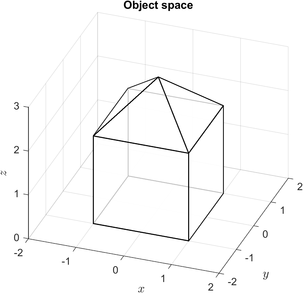
Exercise 17

The diagram belows shows the side view and a plan view of an object.

The object is defined in the object space so that the centre of the base it as the origin. Define the vertex and face matrices in MATLAB and produce a plot of the object space.

Solution to Exercise 17

% Define object
Vobj = [ -1,  1,  1, -1, -1,  1,  1, -1,  0 ;
         -1, -1,  1,  1, -1, -1,  1,  1,  0 ;
          0,  0,  0,  0,  2,  2,  2,  2,  3 ;
          1,  1,  1,  1,  1,  1,  1,  1,  1];
Fobj = [ 4, 3, 2, 1 ;
         1, 2, 6, 5 ;
         2, 3, 7, 6 ;
         3, 4, 8, 7 ;
         5, 8, 4, 1 ;
         6, 5, 9, 9 ;
         6, 7, 9, 9 ;
         7, 8, 9, 9 ;
         8, 5, 9, 9 ];

% Plot object space
figure
patch('Vertices', Vobj(1:3,:)', 'Faces', Fobj, FaceColor='white', FaceAlpha=0.75, LineWidth=2)
title('Object space')
xlabel('$x$', 'Interpreter', 'latex', 'FontSize', 12)
ylabel('$y$', 'Interpreter', 'latex', 'FontSize', 12)
zlabel('$z$', 'Interpreter', 'latex', 'FontSize', 12)
view(30, 30)
axis equal
axis([-2, 2, -2, 2, 0, 3])
grid on 

Exercise 18

The object from Exercise 17 is used to build a virtual environment consisting of two objects. The first object is scaled by 0.5 in the \(x\) and \(y\) directions and 2 in the \(z\) direction, rotated about the \(z\)-axis by angle \(\pi/3\) and translated so that the centre of the base of the object is at \((3, 3, 0)\). The second object is scaled by 2 in the \(y\) direction, rotated by angle \(\pi/4\) about the \(z\)-axis and translated so that the centre of the base of the object is at \((6, 6, 0)\).

In MATLAB, determine the world space vertex and face matrices and produce a plot of the world space.

Solution to Exercise 18

% Define object positions, scaling and rotations
pos = [ 3, 3, 0 ;
        6, 6, 0 ];
scale = [ 0.5, 0.5, 2 ;
          1,   2,   1 ];
angle = [ 0, 0, pi/3 ;
          0, 0, pi/4 ];

% Define transformation matrices
T = @(t) [ 1, 0, 0, t(1) ;
           0, 1, 0, t(2) ;
           0, 0, 1, t(3) ;
           0, 0, 0, 1 ];
           
S = @(s) [ s(1), 0, 0, 0 ;
           0, s(2), 0, 0 ;
           0, 0, s(3), 0 ;
           0, 0, 0, 1 ];

Rx = @(theta) [ 1, 0, 0, 0 ;
                0, cos(theta), -sin(theta), 0 ;
                0, sin(theta), cos(theta), 0 ;
                0, 0, 0, 1 ];

Ry = @(theta) [ cos(theta), 0, sin(theta), 0 ;
                0, 1, 0, 0 ;
                -sin(theta), 0, cos(theta), 0 ;
                0, 0, 0, 1 ];

Rz = @(theta) [ cos(theta), -sin(theta), 0, 0 ;
                sin(theta), cos(theta), 0, 0 ;
                0, 0, 1, 0 ;
                0, 0, 0, 1 ];

% Loop through objects
Vworld = [];
Fworld = [];
for i = 1 : 2

    % Get object vertices and face array
    Vobj = V;
    Fobj = F + size(Vworld,2);

    % Transform object
    Vobj = T(pos(i,:)) * Rx(angle(i,1)) * Ry(angle(i,2)) * Rz(angle(i,3)) * S(scale(i,:)) * V;

    % Add object to world space
    Vworld = [Vworld, Vobj];
    Fworld = [Fworld ; Fobj];
end

% Plot world space
figure
patch('Vertices', Vworld(1:3,:)', 'Faces', Fworld, FaceColor='white', FaceAlpha=0.75, LineWidth=1)
title('World space')
xlabel('$x$', 'Interpreter', 'latex', 'FontSize', 12)
ylabel('$y$', 'Interpreter', 'latex', 'FontSize', 12)
zlabel('$z$', 'Interpreter', 'latex', 'FontSize', 12)
view(30, 30)
axis equal
axis([0, 10, 0, 10, 0, 6])
grid on 

Exercise 19

The world space from Exercise 18 is to be viewed from the position \((12, 7, 4)\) looking towards the centre of view at \((5, 5, 2)\). Calculate the camera space co-ordinates and produce a plot of the camera space looking down the \(z\)-axis.

Solution to Exercise 19

% Define viewing position and centre of view
p = [12 , 7 , 4];
c = [5 , 5 , 2];
k = [0 , 0 , 1];

% Calculate alignment matrix
w = (p - c) / norm(p - c);
u = cross(k, w) / norm(cross(k, w));
v = cross(w, u);
A = [ u, -dot(p, u) ; 
      v, -dot(p, v) ;
      w, -dot(p, w) ;
      0, 0, 0, 1 ];

% Align world space to the camera space
Vcamera = A * Vworld;

%Plot camera space
figure
h1 = axes;
patch("Vertices", Vcamera([1,3,2],:)', "Faces", Fworld, FaceColor="w", FaceAlpha=0.75, LineWidth=1)
hold on
plot3(0, 0, 0, "bo", MarkerFaceColor="b")
quiver3(0, 0, 0, 0, -1, 0, "b", MaxHeadSize=1)
hold off
set(h1, "Ydir", "reverse")  % reverse z axis so that it matches the right-hand rule
title('Camera space')
xlabel("$x$", "Interpreter", "latex", "FontSize", 12)
ylabel("$z$", "Interpreter", "latex", "FontSize", 12)
zlabel("$y$", "Interpreter", "latex", "FontSize", 12)
view(0,0)
axis([-5, 5, -15, 0, -5, 5])

Exercise 20

The camera space from Exercise 19 is projected onto a screen space defined by the near and far viewing planes at distances 2 and 10 away from the origin respectively, a field of view angle \(\pi/3\) and an aspect ratio of \(4:3\). Calculate the screen space co-ordinates and produce a plot of the screen space looking down the \(z\)-axis.

Solution to Exercise 20

near = 2;
far = 10;
fov = pi/3;
aspect = 4/3;

% Calculate projection matrix
r = near * tan(fov / 2);
t = r / aspect;
P = [-near / r, 0, 0, 0 ;
     0, -near / t, 0, 0 ;
     0, 0, (near + far) / (near - far), 2 * near * far / (near - far) ;
     0, 0, 1, 0 ];

% Calculate screen space co-ordinates
Vscreen = P * Vcamera;
Vscreen = Vscreen ./ Vscreen(4,:);

% Plot screen space viewed from the side
figure()
h1 = axes;
patch("Vertices", Vscreen([1,3,2],:)', "Faces", Fworld, FaceColor="w", FaceAlpha=0.75, LineWidth=1)
hold on
plot3(0, 1, 0,"bo",MarkerFaceColor="b")
quiver3(0, 1, 0, 0, -0.5, 0, "b", MaxHeadSize=1)
hold off
title('Screen space')
xlabel("$x$", "Interpreter", "latex", "FontSize", 18)
ylabel("$z$", "Interpreter", "latex", "FontSize", 18)
zlabel("$y$", "Interpreter", "latex", "FontSize", 18)
set(h1, "Ydir", "reverse")  % reverse z axis so that it matches the right-hand rule
view(0,0)
axis([-1.2, 1.2, -1.2, 1.2, -1.2, 1.2])