World space

Once the objects have been define they can be used to build the virtual environment. The objects are copied to the world space and transformed using scaling, rotation and translation operations to construct the virtual world.

Fig. 57 The world space

The transformations applied to the objects is done in the order scaling followed by rotation followed by translation so that the shape of the object is preserved. Therefore the world space vertices of each object vertices are calculated using

\[ \begin{align*} V_{\text{object}} = T \cdot R_z \cdot R_y \cdot R_x \cdot S \cdot V. \end{align*} \]

The object vertex co-ordinates are then appended to a vertex matrix containing all of the objects in the virtual environment, i.e.,

\[ \begin{align*} V_{\text{world}} = \begin{pmatrix} V_{\text{object 1}} & V_{\text{object 2}} & V_{\text{object 3}} & \cdots &\end{pmatrix}. \end{align*} \]

So \(V_{\text{world}}\) is a \(4 \times N_{verts}\) matrix where \(N_{verts}\) is the total number of vertices that define the virtual environment. The face array for each object is also appended to the bottom of a face matrix containing all faces for the objects that make up the virtual environment, i.e.,

\[\begin{split} \begin{align*} F_{\text{world}} = \begin{pmatrix} F_{\text{obj1}} \\ F_{\text{obj2}} \\ \vdots \end{pmatrix}. \end{align*} \end{split}\]

So \(F_{\text{world}}\) is an \(N_{faces} \times N_{sides}\) matrix where \(N_{faces}\) is the total number of faces in the virtual environment and \(N_{sides}\) is the maximum number of sides of the faces. Since \(F_{\text{world}}\) links to \(V_{\text{world}}\) then when adding a new face to \(F_{\text{world}}\) we need to add the number of columns currently in \(V_{\text{world}}\) to \(F_{\text{object}}\).

Example 30

The virtual world shown in figure Fig. 57 is constructed using 2 house objects from Example 29 and a cube object. The house objects are rotated by angle \(\theta = \pi/2\) about the \(z\) axis and translated so that the centre of the bases have position vectors \(\mathbf{c}_1 = (3, 3.5, 0)\) and \(\mathbf{c}_2 = (3, 1.5, 0)\). The cube object has side lengths 2 is scaled by a factor of \(0.5\) in the \(x\) and \(y\) directions and \(1.5\) in the \(z\) direction so that it resembles a tower and translated so that the centre of the base is at \(\mathbf{c}_3 = (1.5, 1.5, 0)\). Determine the vertex and face matrices for the world space.

Solution

Since \(\cos(\pi/2) = 0\) and \(\sin(\pi/2) = 1\) then the rotation and translation matrices for the first house object are

\[\begin{split} \begin{align*} R_z(\theta) &= \begin{pmatrix} 0 & -1 & 0 & 0 \\ 1 & 0 & 0 & 0 \\ 0 & 0 & 1 & 0 \\ 0 & 0 & 0 & 1 \end{pmatrix}, & T(\mathbf{c}_1) &= \begin{pmatrix} 1 & 0 & 0 & 3 \\ 0 & 1 & 0 & 3.5 \\ 0 & 0 & 1 & 0 \\ 0 & 0 & 0 & 1 \end{pmatrix} \end{align*} \end{split}\]

so the composite transformation matrix is

\[\begin{split} \begin{align*} A &= T(\mathbf{c}_1) \cdot R_z(\theta) = \begin{pmatrix} 0 & -1 & 0 & 3 \\ 1 & 0 & 0 & 3.5 \\ 0 & 0 & 1 & 0 \\ 0 & 0 & 0 & 1 \end{pmatrix}. \end{align*} \end{split}\]

Applying the composite transformation to \(V_{\text{house}}\) from Example 29 gives

\[\begin{split} \begin{align*} V_{\text{world}} &= \begin{pmatrix} 0 & -1 & 0 & 3 \\ 1 & 0 & 0 & 3.5 \\ 0 & 0 & 1 & 0 \\ 0 & 0 & 0 & 1 \end{pmatrix} \begin{pmatrix} -0.5 & 0.5 & 0.5 & -0.5 & -0.5 & 0.5 & 0.5 & -0.5 & 0 & 0 \\ -1 & -1 & 1 & 1 & -1 & -1 & 1 & 1 & -1 & 1 \\ 0 & 0 & 0 & 0 & 1 & 1 & 1 & 1 & 2 & 2 \\ 1 & 1 & 1 & 1 & 1 & 1 & 1 & 1 & 1 & 1 \end{pmatrix} \\ &= \begin{pmatrix} 2 & 2 & 4 & 4 & 2 & 2 & 4 & 4 & 2 & 4 \\ 3 & 4 & 4 & 3 & 3 & 4 & 4 & 3 & 3.5 & 3.5 \\ 0 & 0 & 0 & 0 & 1 & 1 & 1 & 1 & 2 & 2 \\ 1 & 1 & 1 & 1 & 1 & 1 & 1 & 1 & 1 & 1 \end{pmatrix}, \end{align*} \end{split}\]

and since this is the first object added to the world space then \(F_{\text{world}} = F_{\text{house}}\). Doing similar for the second house object gives the following composite transformation matrix

\[\begin{split} \begin{align*} T(\mathbf{c}_1) \cdot R_z(\theta) &= \begin{pmatrix} 0 & -1 & 0 & 3 \\ 1 & 0 & 0 & 1.5 \\ 0 & 0 & 1 & 0 \\ 0 & 0 & 0 & 1 \end{pmatrix} \end{align*} \end{split}\]

which applied to the object co-ordinates for the house object gives

\[\begin{split} \begin{align*} T \cdot S \cdot V_{\text{house}} = \begin{pmatrix} 2 & 2 & 4 & 4 & 2 & 2 & 4 & 4 & 2 & 4 \\ 1 & 2 & 2 & 1 & 1 & 2 & 2 & 1 & 1.5 & 1.5 \\ 0 & 0 & 0 & 0 & 1 & 1 & 1 & 1 & 2 & 2 \\ 1 & 1 & 1 & 1 & 1 & 1 & 1 & 1 & 1 & 1 \end{pmatrix}, \end{align*} \end{split}\]

These are appended to the end of the world space vertex matrix

\[\begin{split} \begin{align*} V_{\text{world}} &= \begin{matrix} \left( \begin{matrix} 2 & 2 & \cdots & 4 \\ 1 & 2 & \cdots & 3.5 \\ 0 & 0 & \cdots & 2 \\ 1 & 1 & \cdots & 1 \end{matrix} \right. & \quad \left. \begin{matrix} 2 & 2 & \cdots & 4 \\ 1 & 2 & \cdots & 1.5 \\ 0 & 0 & \cdots & 2 \\ 1 & 1 & \cdots & 1 \end{matrix} \right) \\ \textsf{house 1} & \textsf{house 2} \end{matrix}. \end{align*} \end{split}\]

Since the the number of vertices was \(N_{verts} = 10\) prior to appending the second house object then we need to add 10 to \(F_{\text{house}}\) and append it to \(F_{\text{world}}\)

\[\begin{split} \begin{align*} F_{\text{world}} &= \begin{pmatrix} 1 & 4 & 3 & 2 & 2 \\ 1 & 2 & 6 & 9 & 5 \\ \vdots & \vdots & \vdots & \vdots & \vdots \\ 5 & 9 & 10 & 8 & 8 \\ 11 & 14 & 13 & 12 & 12 \\ 11 & 12 & 16 & 19 & 15 \\ \vdots & \vdots & \vdots & \vdots & \vdots \\ 15 & 19 & 20 & 18 & 18 \end{pmatrix}. \end{align*} \end{split}\]

The scaling and translation matrices for the cube (tower) object are

\[\begin{split} \begin{align*} S &= \begin{pmatrix} 0.5 & 0 & 0 & 0 \\ 0 & 0.5 & 0 & 0 \\ 0 & 0 & 1.5 & 0 \\ 0 & 0 & 0 & 1 \end{pmatrix}, & T &= \begin{pmatrix} 1 & 0 & 0 & 1.5 \\ 0 & 1 & 0 & 1.5 \\ 0 & 0 & 1 & 1.5 \\ 0 & 0 & 0 & 1 \end{pmatrix}, \end{align*} \end{split}\]

which gives the transformed vertex matrix

\[\begin{split} \begin{align*} T(\mathbf{c}_3) \cdot S(\mathbf{s}) \cdot V_{\text{cube}} = \begin{pmatrix} 1 & 2 & 2 & 1 & 1 & 2 & 2 & 1 \\ 1 & 1 & 2 & 2 & 1 & 1 & 2 & 2 \\ 0 & 0 & 0 & 0 & 3 & 3 & 3 & 3 \\ 1 & 1 & 1 & 1 & 1 & 1 & 1 & 1 \end{pmatrix}. \end{align*} \end{split}\]

Appending these to \(V_{\text{world}}\) gives

\[\begin{split} \begin{align*} V_{\text{world}} &= \begin{matrix} \left( \begin{matrix} 2 & 2 & \cdots & 4 \\ 2 & 1 & \cdots & 1.5 \\ 0 & 0 & \cdots & 2 \\ 1 & 1 & \cdots & 1 \end{matrix} \right. & \quad & \left. \begin{matrix} 1 & 2 & \cdots & 1 \\ 1 & 1 & \cdots & 2 \\ 0 & 0 & \cdots & 3 \\ 1 & 1 & \cdots & 1 \end{matrix} \right) \\ \textsf{world space} & & \textsf{tower object} \end{matrix}. \end{align*} \end{split}\]

There were \(N_{verts}=20\) vertices in the world space prior to appending the cube object so we need to add 20 to \(F_{\text{cube}}\) and append it to \(F_{\text{world}}\)

\[\begin{split} \begin{align*} F_{\text{world}} = \begin{pmatrix} 1 & 4 & 3 & 2 & 2 \\ 1 & 2 & 6 & 9 & 5 \\ \vdots & \vdots & \vdots & \vdots & \vdots \\ 15 & 19 & 20 & 18 & 18 \\ 21 & 24 & 23 & 22 & 22\\ 21 & 22 & 26 & 25 & 25 \\ \vdots & \vdots & \vdots & \vdots & \vdots \\ 25 & 26 & 27 & 28 & 28 \end{pmatrix}. \end{align*} \end{split}\]

After the 3 objects have been added to the world space the virtual world is described by 20 polygons defined by 28 vertices.

MATLAB code

The MATLAB code below defines the vertex and face matrix for a cube object as well as the world space objects, positions, scales and angles for the virtual world from Example 30.

% Define cube object
Vcube = [ -1,  1,  1, -1, -1,  1, 1, -1 ;
          -1, -1,  1,  1, -1, -1, 1,  1 ;
          -1, -1, -1, -1,  1,  1, 1,  1 ;
           1,  1,  1,  1,  1,  1, 1,  1 ];

Fcube = [ 1, 4, 3, 2, 2 ;
          1, 2, 6, 5, 5 ; 
          2, 3, 7, 6, 6 ;
          3, 4, 8, 7, 7 ;
          4, 1, 5, 8, 8 ;
          5, 6, 7, 8, 8 ];

% Define object types, positions, scaling and rotation angles
object = [ 2, 2, 1 ];        % object types (1 = cube, 2 = house)
pos = [ 3,   3.5, 0 ;        % object positions (x, y, z)
        3,   1.5, 0 ;
        1.5, 1.5, 1.5 ];
scale = [ 1,   1,   1 ;      % object scales (sx, sy, sz)
          1,   1,   1 ;
          0.5, 0.5, 1.5 ];
angle = [ 0, 0, pi/2 ;       % object angles (theta_x, theta_y, theta_z)
          0, 0, pi/2 ;
          0, 0, 0 ];

We will be using translation, scaling and rotation transformations on our objects so these are defined below.

% Define transformation matrices
T = @(t) [ 1, 0, 0, t(1) ; 
           0, 1, 0, t(2) ; 
           0, 0, 1, t(3) ; 
           0, 0, 0, 1 ];

S = @(s) [ s(1), 0,    0,    0 ;  
           0,    s(2), 0,    0 ; 
           0,    0,    s(3), 0 ; 
           0,    0,    0,    1 ];

Rx = @(theta) [ 1, 0, 0, 0 ;
                0, cos(theta), -sin(theta), 0 ;
                0, sin(theta), cos(theta), 0 ;
                0, 0, 0, 1];

Ry = @(theta) [ cos(theta), 0, sin(theta), 0 ;
                0, 1, 0, 0 ;
                -sin(theta), 0, cos(theta), 0 ;
                0, 0, 0, 1 ];

Rz = @(theta) [ cos(theta), -sin(theta), 0, 0 ;
                sin(theta), cos(theta), 0, 0 ;
                0,           0,         1, 0 ;
                0,           0,         0, 1 ];

We can now build the world space. Here we loop through the three objects and depending on the value of object(i) we determine the vertex and face matrix for the object. It is then transformed using the values of the position pos(i,:), rotation angles angle(i,:) and scales scale(i,:) for the object. We also add the number of vertices currently in the world space matrix Vworld to the face matrix. The transformed object vertices and face matrices are appended to Vworld and Fworld.

% Add objects to world space
Vworld = [];
Fworld = [];
for i = 1 : 3

    % Get object vertices and face array
    if object(i) == 1  % cube object
        Vobj = Vcube;
        Fobj = Fcube + size(Vworld,2);  % add number of vertices in the world space to F
    elseif object(i) == 2  % house object
        Vobj = Vhouse;
        Fobj = Fhouse + size(Vworld,2);
    end

    % Transform object
    Vobj = T(pos(i,:)) * Rx(angle(i,1)) * Ry(angle(i,2)) * Rz(angle(i,3)) * S(scale(i,:)) * Vobj;

    % Add object to world space
    Vworld = [Vworld, Vobj];
    Fworld = [Fworld ; Fobj];
end

The MATLAB code below plots the world space. This is similar to the code used to plot the object space.

% Plot world space
figure
patch("Vertices", Vworld(1:3,:)', "Faces", Fworld, FaceColor="w", FaceAlpha=0.75, LineWidth=1)
title('World space')
xlabel("$x$", "Interpreter", "latex", "FontSize", 12)
ylabel("$y$", "Interpreter", "latex", "FontSize", 12)
zlabel("$z$", "Interpreter", "latex", "FontSize", 12)
view(60, 30)
axis([0, 5, 0, 5, 0, 4])
grid on

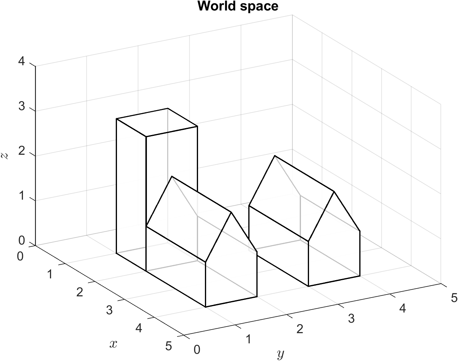
Fig. 58 The world space from Example 30.