Week 8 — Matrix Decomposition II

6G6Z3017 Computational Methods in ODEs

Dr Jon Shiach

QR Decomposition

QR decomposition is another decomposition method that factorises a matrix in the product of two matrices \(Q\) and \(R\) such that

\[ \begin{align*} A = QR, \end{align*} \]

where \(Q\) is an orthogonal matrix and \(R\) is an upper triangular matrix.

Note

A set of vectors \(\lbrace \mathbf{v}_1 ,\mathbf{v}_2 ,\mathbf{v}_3 ,\dots \rbrace\) is said to be orthogonal if \(\mathbf{v}_i \cdot \mathbf{v}_j =0\) for \(i\not= j\). Furthermore the set is said to be orthonormal if \(\mathbf{v}_i\) are all unit vectors.

Note

An orthogonal matrix is a matrix where the columns are a set of orthonormal vectors. If \(A\) is an orthogonal matrix if

\[ \begin{align*} A^\mathsf{T} A=I. \end{align*} \]

Consider the matrix

\[ \begin{align*} A= \begin{pmatrix} 0.8 & -0.6\\ 0.6 & 0.8 \end{pmatrix}. \end{align*} \]

This is an orthogonal matrix since

\[ \begin{align*} A^\mathsf{T} A=\begin{pmatrix} 0.8 & 0.6\\ -0.6 & 0.8 \end{pmatrix} \begin{pmatrix} 0.8 & -0.6\\ 0.6 & 0.8 \end{pmatrix} = \begin{pmatrix} 1 & 0\\ 0 & 1 \end{pmatrix}=I. \end{align*} \]

Furthermore it is an orthonormal matrix since the magnitude of the columns for \(A\) are both 1.

QR decomposition using the Gram-Schmidt process

Consider the \(3 \times 3\) matrix \(A\) represented as the concatenation of the column vectors \(\mathbf{a}_1, \mathbf{a}_2, \mathbf{a}_3\)

\[ \begin{pmatrix} a_{11} & a_{12} & a_{13} \\ a_{21} & a_{22} & a_{23} \\ a_{31} & a_{32} & a_{33} \end{pmatrix} = \begin{pmatrix} \uparrow & \uparrow & \uparrow \\ \mathbf{a}_1 & \mathbf{a}_2 & \mathbf{a}_3 \\ \downarrow & \downarrow & \downarrow \end{pmatrix} \]

To calculate the orthogonal \(Q\) matrix we need a set of vectors \(\{\mathbf{q}_1, \mathbf{q}_2, \mathbf{q}_3\}\) that span the same space as \(\{\mathbf{a}_1, \mathbf{a}_2, \mathbf{a}_3\}\) but are orthogonal to each other. One way to do this is using the Gram-Schmidt process.

The Gram-Schmidt Process

Consider this diagram that shows the first two non-orthogonal vectors \(\mathbf{a}_1\) and \(\mathbf{a}_2\).

The Gram-Schmidt Process

\(\mathbf{q}_1\) is the unit vector that is parallel to \(\mathbf{a}_1\)

The Gram-Schmidt Process

\((\mathbf{a}_2 \cdot \mathbf{q}_1) \mathbf{q}_1\) is the vector projection of \(\mathbf{a}_2\) onto \(\mathbf{a}_1\).

The Gram-Schmidt Process

Subracting this projection from \(\mathbf{a}_2\) gives the orthogonal vector \(\mathbf{u}_2\).

The Gram-Schmidt Process

Subracting this projection from \(\mathbf{a}_2\) gives the orthogonal vector \(\mathbf{u}_2\).

The Gram-Schmidt Process

Normalising \(\mathbf{u}_2\) gives the unit orthogonal vector \(\mathbf{q}_2\).

QR decomposition using the Gram-Schmidt process

Subtract the vector projection of \(\mathbf{a}_2\) onto \(\mathbf{u}_1\)

\[ \mathbf{u}_2 = \mathbf{a}_2 - \left( \frac{\mathbf{q}_1 \cdot \mathbf{a}_1}{\mathbf{q}_1 \cdot \mathbf{u}_1} \right) \mathbf{u}_1.\]

Normalise \(\mathbf{u}_1\) such that \(\mathbf{q}_1 = \dfrac{\mathbf{u}_1}{\|\mathbf{u}_1\|}\) so we have

\[ \mathbf{u}_2 = \mathbf{a}_2 - (\mathbf{q}_1 \cdot \mathbf{a}_2) \mathbf{q}_1. \]

Normalise \(\mathbf{u}_2\) to give \(\mathbf{q}_2 = \dfrac{\mathbf{u}_2}{\|\mathbf{u}_2\|}\).

Subtract the vector projections of \(\mathbf{a}_3\) onto \(\mathbf{q}_1\) and \(\mathbf{q}_2\) from \(\mathbf{a}_3\)

\[ \mathbf{u}_3 = \mathbf{a}_3 - (\mathbf{q}_1 \cdot \mathbf{a}_3) \mathbf{q}_1 - (\mathbf{q}_2 \cdot \mathbf{a}_3) \mathbf{q}_2. \]

Normalise \(\mathbf{u}_3\) to give \(\mathbf{q}_3 = \dfrac{\mathbf{u}_3}{\|\mathbf{u}_3\|}\).

Since \(\mathbf{u}_i = (\mathbf{q}_i \cdot \mathbf{a}_i) \mathbf{q}_i\) and rearranging the equations for \(\mathbf{u}_i\) to make \(\mathbf{a}_i\) the subject gives

\[ \begin{align*} \mathbf{a}_1 &= (\mathbf{q}_1 \cdot \mathbf{a}_1), \\ \mathbf{a}_2 &= (\mathbf{q}_1 \cdot \mathbf{a}_2) \mathbf{q}_1 + (\mathbf{q}_2 \cdot \mathbf{a}_2) \mathbf{q}_2, \\ \mathbf{a}_3 &= (\mathbf{q}_1 \cdot \mathbf{a}_3) \mathbf{q}_1 + (\mathbf{q}_2 \cdot \mathbf{a}_3) \mathbf{q}_2 + (\mathbf{q}_3 \cdot \mathbf{a}_3) \mathbf{q}_3, \\ & \vdots \end{align*} \]

The columns of the \(Q\) matrix are formed using the vectors \(\mathbf{q}_i\)

\[ Q = \begin{pmatrix} \uparrow & \uparrow & & \uparrow \\ \mathbf{q}_1 & \mathbf{q}_2 & \cdots & \mathbf{q}_n \\ \downarrow & \downarrow & & \downarrow \end{pmatrix}, \]

and the elements of the \(R\) matrix are formed from the dot products of the \(\mathbf{q}_i\) and \(\mathbf{a}_j\) vectors such that

\[ R = \begin{pmatrix} (\mathbf{q}_1 \cdot \mathbf{a}_1) & (\mathbf{q}_1 \cdot \mathbf{a}_2) & \cdots & (\mathbf{q}_1 \cdot \mathbf{a}_n) \\ 0 & (\mathbf{q}_2 \cdot \mathbf{a}_2) & \cdots & (\mathbf{q}_1 \cdot \mathbf{a}_n) \\ \vdots & \ddots & \ddots & \vdots \\ 0 & \cdots & 0 & (\mathbf{q}_n \cdot \mathbf{a}_n) \end{pmatrix}. \]

QR Gram-Schmidt Algorithm

Note

For \(j = 1, \ldots, n\) do
- For \(i = 1, \ldots, j - 1\) do
  - \(r_{ij} \gets \mathbf{q}_i \cdot \mathbf{a}_j\)
- \(\mathbf{u}_j \gets \mathbf{a}_j - \displaystyle\sum_{i=1}^{j-1} r_{ij} \mathbf{q}_j\)
- \(r_{jj} \gets \| \mathbf{u}_j \|\)
- \(\mathbf{q}_j \gets \dfrac{\mathbf{u}_j}{r_{jj}}\)
\(Q \gets (\mathbf{q}_1, \mathbf{q}_2, \ldots, \mathbf{q}_2)\)
For \(i = 1, \ldots, n\) do
- If \(r_{ii} < 0\) then
  - \(R(i,: ) \gets -R(i,:)\)
  - \(Q(:,i) \gets -Q(:,i)\)

QR Gram-Schmidt Example

Calculate the QR decomposition of the following matrix using the Gram-Schmidt process

\[ \begin{align*} A = \begin{pmatrix} -1 & -1 & 1 \\ 1 & 3 & 3 \\ -1 & -1 & 5 \\ 1 & 3 & 7 \end{pmatrix}. \end{align*} \]

Solution:

\[ \begin{align*} j &= 1: & \mathbf{u}_1 &= \mathbf{a}_1 = \begin{pmatrix} -1 \\ 1 \\ -1 \\ 1 \end{pmatrix}, \\ && r_{11} &= \| \mathbf{u}_1 \| = 2, \\ && \mathbf{q}_1 &= \frac{\mathbf{u}_1}{r_{11}} = \frac{1}{2} \begin{pmatrix} -1 \\ 1 \\ 1 \\ 1 \end{pmatrix} = \begin{pmatrix} -\frac{1}{2} \\ \frac{1}{2} \\ -\frac{1}{2} \\ \frac{1}{2} \end{pmatrix}, \\ \end{align*} \]

\[ \begin{align*} j &= 2: & r_{12} &= \mathbf{q}_1 \cdot \mathbf{a}_2 = \begin{pmatrix} -\frac{1}{2} \\ \frac{1}{2} \\ -\frac{1}{2} \\ \frac{1}{2} \end{pmatrix} \cdot \begin{pmatrix} -1 \\ 3 \\ -1 \\ 3 \end{pmatrix} = 4, \\ && \mathbf{u}_2 &= \mathbf{a}_2 - r_{12} \mathbf{q}_1 = \begin{pmatrix} -1 \\ 3 \\ -1 \\ 3 \end{pmatrix} - 4 \begin{pmatrix} -\frac{1}{2} \\ \frac{1}{2} \\ -\frac{1}{2} \\ \frac{1}{2} \end{pmatrix} = \begin{pmatrix} 1 \\ 1 \\ 1 \\ 1 \end{pmatrix}, \\ && r_{22} &= \| \mathbf{u}_2 \| = 2, \\ && \mathbf{q}_2 &= \frac{\mathbf{u}_2}{r_{22}} = \frac{1}{2} \begin{pmatrix} 1 \\ 1 \\ 1 \\ 1 \end{pmatrix} = \begin{pmatrix} \frac{1}{2} \\ \frac{1}{2} \\ \frac{1}{2} \\ \frac{1}{2} \end{pmatrix}. \end{align*} \]

The diagonal elements of \(R\) are all positive so we don’t need to make any adjustments. Thus the \(Q\) and \(R\) matrices are given by

\[ \begin{align*} Q &= \begin{pmatrix} -\frac{1}{2} & \frac{1}{2} & -\frac{1}{2} \\ \frac{1}{2} & \frac{1}{2} & -\frac{1}{2} \\ -\frac{1}{2} & \frac{1}{2} & \frac{1}{2} \\ \frac{1}{2} & \frac{1}{2} & \frac{1}{2} \end{pmatrix}, & R &= \begin{pmatrix} 2 & 4 & 2 \\ 0 & 2 & 8 \\ 0 & 0 & 4 \end{pmatrix}. \end{align*} \]

We can check that this is correct by verifying that \(A = QR\) and that \(Q^\mathsf{T}Q = I\).

\[ \begin{align*} \begin{pmatrix} -\frac{1}{2} & \frac{1}{2} & -\frac{1}{2} \\ \frac{1}{2} & \frac{1}{2} & -\frac{1}{2} \\ -\frac{1}{2} & \frac{1}{2} & \frac{1}{2} \\ \frac{1}{2} & \frac{1}{2} & \frac{1}{2} \end{pmatrix} \begin{pmatrix} 2 & 4 & 2 \\ 0 & 2 & 8 \\ 0 & 0 & 4 \end{pmatrix} &= \begin{pmatrix} -1 & -1 & 1 \\ 1 & 3 & 3 \\ -1 & -1 & 5 \\ 1 & 3 & 7 \end{pmatrix} = A, \\ \begin{pmatrix} -\frac{1}{2} & \frac{1}{2} & -\frac{1}{2} & \frac{1}{2} \\ \frac{1}{2} & \frac{1}{2} & \frac{1}{2} & \frac{1}{2} \\ -\frac{1}{2} & -\frac{1}{2} & \frac{1}{2} & \frac{1}{2} \end{pmatrix} \begin{pmatrix} -\frac{1}{2} & \frac{1}{2} & -\frac{1}{2} \\ \frac{1}{2} & \frac{1}{2} & -\frac{1}{2} \\ -\frac{1}{2} & \frac{1}{2} & \frac{1}{2} \\ \frac{1}{2} & \frac{1}{2} & \frac{1}{2} \end{pmatrix} &= \begin{pmatrix} 1 & 0 & 0 \\ 0 & 1 & 0 \\ 0 & 0 & 1 \end{pmatrix} = I. \end{align*} \]

Householder Reflections

A Householder reflection reflects a vector \(\mathbf{x}\) about a hyperplane that is orthogonal to a given vector \(\mathbf{v}\).

The Householder matrix is an orthogonal reflection matrix of the form

\[ H = I - 2 \frac{\mathbf{v} \mathbf{v}^\mathsf{T}}{\mathbf{v}^\mathsf{T} \mathbf{v}}. \]

where \(\mathbf{v} = \mathbf{x} - \| \mathbf{x} \| \mathbf{e}_1\).

The matrix \(H\) is symmetric and orthogonal.

If the magnitude of \(\mathbf{x}\) is close to being parallel to \(\mathbf{e}_1\) then the calculation of \(\mathbf{v}\) will involve the division by a number close to zero.

To overcome this we use a Householder transformation to reflect \(\mathbf{x}\) so that it is parallel to \(-\mathbf{e}_1\) instead of \(+\mathbf{e}_1\).

To do this we calculate \(\mathbf{v}\) by adding \(\| \mathbf{x} \| \mathbf{e}_1\) to \(\mathbf{x}\) when the sign of \(x_1\) is negative, i.e.,

\[ \mathbf{v} = \mathbf{x} - \operatorname{sign}(x_1) \| \mathbf{x} \| \mathbf{e}_1, \]

where \(\operatorname{sign}(x)\) returns \(+1\) if \(x \geq 0\) and \(-1\) if \(x < 0\).

QR Decomposition using Householder Reflections

To compute the QR decomposition of a matrix \(A\), we reflect the first column of \(A\), using Householder reflection so that it is parallel to \(\mathbf{e}_1\).

The vector \(\mathbf{v}\) is given by

\[ \mathbf{v} = \mathbf{x} - \operatorname{sign}(x_1) \|\mathbf{x}\| \mathbf{e}_1, \]

where \(\mathbf{x}\) is the first column of \(A\) and \(\mathbf{e}_1 = (1, 0, \ldots, 0)^\mathsf{T}\) is the first basis vector.

The first Householder matrix is then given by

\[ H_1 = I - 2 \frac{\mathbf{v} \mathbf{v}^\mathsf{T}}{\mathbf{v}^\mathsf{T} \mathbf{v}}. \]

Multiplying \(H_1\) by \(A\) reflects the first column of \(A\) such that it is parallel to \(\mathbf{e}_1\).

\[ \begin{align*} R = H_1 A = \begin{pmatrix} r_{11} & r_{12} & r_{13} & \cdots & r_{1n} \\ 0 & b_{22} & b_{23} & \cdots & b_{2n} \\ 0 & b_{32} & b_{33} & \cdots & b_{3n} \\ \vdots & \vdots & \vdots & \ddots & \vdots \\ 0 & b_{m2} & b_{m3} & \cdots & b_{mn} \end{pmatrix} \end{align*} \]

The second Householder reflection is formed by calculating the Householder matrix \(H'\) using the second column of \(R\) starting from the diagonal element, i.e., \(\mathbf{x} = (b_{22}, b_{32}, \ldots, b_{m2})^\mathsf{T}\).

This is used to form the \(m \times m\) Householder matrix \(H_2\) by padding out the first row and column of the identity matrix.

\[ \begin{align*} H_2 = \begin{pmatrix} 1 & \begin{matrix} 0 & \cdots & 0 \end{matrix} \\ \begin{matrix} 0 \\ \vdots \\ 0 \end{matrix} & H' \end{pmatrix} \end{align*} \]

The Householder matrix \(H_2\) is then applied to \(R\) so that the elements of the second column below the diagonal are zeroed out.

\[ \begin{align*} R = H_2 R = \begin{pmatrix} r_{11} & r_{12} & r_{13} & \cdots & r_{1n} \\ 0 & r_{22} & r_{23} & \cdots & r_{2n} \\ 0 & 0 & c_{33} &\cdots & c_{3n} \\ \vdots & \vdots & \vdots & \ddots & \vdots \\ 0 & 0 & c_{n3} & \cdots & c_{nn} \end{pmatrix} \end{align*} \]

We repeat this process until column \(j = m - 1\) when \(R\) will be an upper triangular matrix. If \(A\) has \(n\) columns then

\[R = H_{m-1}\ldots H_2 H_1 A,\]

rearranging gives

\[\begin{align*} H_1^{-1} H_2^{-1} \ldots H_{m-1}^{-1} R = A. \end{align*} \]

The Householder matrices are symmetric and orthogonal so \(H^{-1} = H\) and since we want \(A = QR\) then

\[ \begin{align*} Q = H_1H_2 \ldots H_{m-1}. \end{align*} \]

QR decomposition using Householder reflections: Aglorithm

Note

\(Q \gets I_m\)
\(R \gets A\)
For \(j = 1, \ldots, m - 1\) do
- \(\mathbf{x} \gets\) column \(j\) of \(R\) starting at the \(j\)-th row
- \(\mathbf{v} \gets \mathbf{x} - \operatorname{sign} (x_1) \|\mathbf{x}\|\mathbf{e}_1\)
- \(H' \gets I_{m-j+1} - 2 \dfrac{\mathbf{v} \mathbf{v} ^\mathsf{T}}{\mathbf{v}^\mathsf{T} \mathbf{v}}\)
- \(H(j:m, j:m) \gets H'\) with the first \(j-1\) rows and columns of \(H\) set to those of \(I_m\)
- \(R \gets H R\)
- \(Q \gets Q H\)
For \(i = 1, \ldots, n\) do
- If \(R(i,i) < 0\) then
  - \(R(i,: ) \gets -R(i,:)\)
  - \(Q(:,i) \gets -Q(:,i)\)

QR Householder Example

Calculate the QR decomposition of the following matrix using Householder reflections

\[ \begin{align*} A=\begin{pmatrix} 1 & -4 \\ 2 & 3 \\ 2 & 2 \end{pmatrix}. \end{align*} \]

Solution:

Set \(Q = I\) and \(R = A\). We want to zero out the elements below \(R(1,1)\) so \(\mathbf{x} = (1, 2, 2)^\mathsf{T}\) and \(\|\mathbf{x}\| = 3\).

\[ \begin{align*} j &= 1: & \mathbf{x} &= \begin{pmatrix} 1 \\ 2 \\ 2 \end{pmatrix}, \\ && \mathbf{v} &= \mathbf{x} - \operatorname{sign}(x_1) \|\mathbf{x}\| \mathbf{e}_1 = \begin{pmatrix} 1 \\ 2 \\ 2 \end{pmatrix} - 3 \begin{pmatrix} 1 \\ 0 \\ 0 \end{pmatrix} = \begin{pmatrix} -2 \\ 2 \\ 2 \end{pmatrix}, \\ && H &= I - 2 \frac{\mathbf{v} \mathbf{v}^\mathsf{T}}{\mathbf{v}^\mathsf{T} \mathbf{v}} = \begin{pmatrix} 1 & 0 & 0 \\ 0 & 1 & 0 \\ 0 & 0 & 1 \end{pmatrix} - \frac{2}{12} \begin{pmatrix} 4 & -4 & -4 \\ -4 & 4 & 4 \\ -4 & 4 & 4 \end{pmatrix} = \begin{pmatrix} \frac{1}{3} & \frac{2}{3} & \frac{2}{3} \\ \frac{2}{3} & \frac{1}{3} & -\frac{2}{3} \\ \frac{2}{3} & -\frac{2}{3} & \frac{1}{3} \end{pmatrix}, \end{align*} \]

\[ \begin{align*} && R &= H R = \begin{pmatrix} \frac{1}{3} & \frac{2}{3} & \frac{2}{3} \\ \frac{2}{3} & \frac{1}{3} & -\frac{2}{3} \\ \frac{2}{3} & -\frac{2}{3} & \frac{1}{3} \end{pmatrix} \begin{pmatrix} 1 & -4 \\ 2 & 3 \\ 2 & 2 \end{pmatrix} = \begin{pmatrix} 3 & 2 \\ 0 & -3 \\ 0 & -4 \end{pmatrix}, \\ && Q &= QH = \begin{pmatrix} 1 & 0 & 0 \\ 0 & 1 & 0 \\ 0 & 0 & 1 \end{pmatrix} \begin{pmatrix} \frac{1}{3} & \frac{2}{3} & \frac{2}{3} \\ \frac{2}{3} & \frac{1}{3} & -\frac{2}{3} \\ \frac{2}{3} & -\frac{2}{3} & \frac{1}{3} \end{pmatrix} = \begin{pmatrix} \frac{1}{3} & \frac{2}{3} & \frac{2}{3} \\ \frac{2}{3} & \frac{1}{3} & -\frac{2}{3} \\ \frac{2}{3} & -\frac{2}{3} & \frac{1}{3} \end{pmatrix}. \end{align*} \]

\[ \begin{align*} j &= 2: & \mathbf{x} &= \begin{pmatrix} -3 \\ -4 \end{pmatrix}, \\ && \mathbf{v} &= \mathbf{x} + \|\mathbf{x}\| \mathbf{e}_1 = \begin{pmatrix} -3 \\ -4 \end{pmatrix} + 5 \begin{pmatrix} 1 \\ 0 \end{pmatrix} = \begin{pmatrix} 2 \\ -4 \end{pmatrix}, \\ && H' &= I - 2 \frac{\mathbf{v}\mathbf{v}^\mathsf{T}}{\mathbf{v}^\mathsf{T} \mathbf{v}} = \begin{pmatrix} 1 & 0 \\ 0 & 1 \end{pmatrix} - \frac{2}{20} \begin{pmatrix} 4 & -8 \\ -8 & 16 \end{pmatrix} = \begin{pmatrix} \frac{3}{5} & \frac{4}{5} \\ \frac{4}{5} & -\frac{3}{5} \end{pmatrix}, \\ && H &= \begin{pmatrix} 1 & 0 & 0 \\ 0 & \frac{3}{5} & \frac{4}{5} \\ 0 & \frac{4}{5} & -\frac{3}{5} \end{pmatrix}, \end{align*} \]

\[ \begin{align*} R &= H R = \begin{pmatrix} 1 & 0 & 0 \\ 0 & -\frac{3}{5} & -\frac{4}{5} \\ 0 & -\frac{4}{5} & \frac{3}{5} \end{pmatrix} \begin{pmatrix} 3 & 2 \\ 0 & 3 \\ 0 & -4 \end{pmatrix} = \begin{pmatrix} 3 & 2 \\ 0 & -5 \\ 0 & 0 \end{pmatrix}, \\ Q &= Q H = \begin{pmatrix} \frac{1}{3} & \frac{2}{3} & \frac{2}{3} \\ \frac{2}{3} & \frac{2}{3} & -\frac{1}{3} \\ \frac{2}{3} & -\frac{1}{3} & \frac{2}{3} \end{pmatrix} \begin{pmatrix} 1 & 0 & 0 \\ 0 & \frac{3}{5} & \frac{4}{5} \\ 0 & \frac{4}{5} & -\frac{3}{5} \end{pmatrix} = \begin{pmatrix} \frac{1}{3} & \frac{14}{15} & \frac{2}{15} \\ \frac{2}{3} & -\frac{1}{3} & \frac{2}{3} \\ \frac{2}{3} & -\frac{2}{15} & -\frac{11}{15} \end{pmatrix}. \end{align*} \]

The second diagonal element of \(R\) is negative, so we multiply row 2 of \(R\) and column 2 of \(Q\) by \(-1\)

\[ \begin{align*} Q &= \begin{pmatrix} \frac{1}{3} & -\frac{14}{15} & \frac{2}{15} \\ \frac{2}{3} & \frac{1}{3} & \frac{2}{3} \\ \frac{2}{3} & \frac{2}{15} & -\frac{11}{15} \end{pmatrix}, & R &= \begin{pmatrix} 3 & 2 \\ 0 & 5 \\ 0 & 0 \end{pmatrix}. \end{align*} \]

We can check whether this is correct by verifying that \(A = QR\) and \(Q^\mathsf{T} Q = I\).

\[ \begin{align*} QR &= \begin{pmatrix} \frac{1}{3} & -\frac{14}{15} & \frac{2}{15} \\ \frac{2}{3} & \frac{1}{3} & \frac{2}{3} \\ \frac{2}{3} & \frac{2}{15} & -\frac{11}{15} \end{pmatrix} \begin{pmatrix} 3 & 2 \\ 0 & 5 \\ 0 & 0 \end{pmatrix} = \begin{pmatrix} 1 & -4 \\ 2 & 3 \\ 2 & 2 \end{pmatrix} = A, \\ Q^\mathsf{T} Q &= \begin{pmatrix} \frac{1}{3} & \frac{2}{3} & \frac{2}{3} \\ -\frac{14}{15} & \frac{1}{3} & \frac{2}{15} \\ \frac{2}{15} & \frac{2}{3} & -\frac{11}{15} \end{pmatrix} \begin{pmatrix} \frac{1}{3} & -\frac{14}{15} & \frac{2}{15} \\ \frac{2}{3} & \frac{1}{3} & \frac{2}{3} \\ \frac{2}{3} & \frac{2}{15} & -\frac{11}{15} \end{pmatrix} = \begin{pmatrix} 1 & 0 & 0 \\ 0 & 1 & 0 \\ 0 & 0 & 1 \end{pmatrix} = I. \end{align*} \]

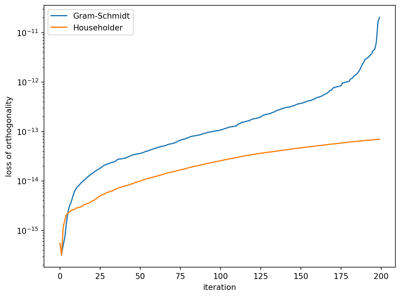
Loss of orthogonality

If \(Q\) is perfectly orthogonal then \(Q^\mathsf{T}Q = I\), but if there is bound to be some small error. If we let this error be \(E\) then \(Q^\mathsf{T}Q = I + E\). Rearranging gives

\[ \| Q^\mathsf{T}Q - I\| = E,\]

which is known as the Frobenius norm and is a measure of the loss of orthogonality.

To analyse the methods, the QR decomposition of a random \(200 \times 200\) matrix \(A\) was computed using the Gram-Schmidt process and Householder reflections.

The Frobenius norm was calculated for the first \(n\) columns of \(Q\) where \(n = 1 \ldots 200\) giving the loss of orthogonality for those iterations.

Eigenvalues

Let \(A\) be an \(n \times n\) matrix then \(\lambda\) is an eigenvalue of \(A\) if there exists a non-zero vector \(\mathbf{v}\) such that

\[A \mathbf{v} = \lambda \mathbf{v}. \qquad(1)\]

The vector \(\mathbf{v}\) is called the eigenvector associated with the eigenvalue \(\lambda\).

Rearranging equation Equation 1 we have

\[ \begin{align*} (A - \lambda I) \mathbf{v} &= \mathbf{0}, \end{align*} \]

which has non-zero solutions for \(\mathbf{v}\) if and only if the determinant of the matrix \((A - \lambda I)\) is zero. Therefore we can calculate the eigenvaleus of \(A\) using

\[ \det(A - \lambda I) = 0.\]

For example, consider the eigenvalues of the matrix

\[ A = \begin{pmatrix} 2 & 1 \\ 2 & 3 \end{pmatrix}.\]

The eigenvalues of \(A\) are given by solving \(\det(A - \lambda I) = 0\) i.e.,

\[ \begin{align*} \det \begin{pmatrix} 2 - \lambda & 1 \\ 2 & 3 - \lambda \end{pmatrix} &= 0 \\ \lambda^2 - 5 \lambda + 4 &= 0 \\ (\lambda - 1)(\lambda - 4) &= 0 \end{align*} \]

so the eigenvalues are \(\lambda_1 = 4\) and \(\lambda_2 = 1\).

The problem with using determinants to calculate eigenvalues is that it is too computationally expensive for larger matrices.

The QR algorithm

Let \(A_0\) be a matrix for which we wish to compute the eigenvalues and \(A_1, \ldots, A_k, A_{k+1}, \ldots\) be a sequence of matrices such that \(A_{k+1} = R_kQ_k\) where \(Q_kR_k = A_k\) is the QR decomposition of \(A_k\).

Since \(Q_k\) is orthogonal then \(Q^{-1} = Q^T\) and

\[ A_{k+1} = R_kQ_k = Q_k^{-1}Q_kR_kQ_k = Q^{-1}A_kQ_k = Q_k^\mathrm{T}A_kQ_k\]

The matrices \(Q_k^\mathrm{T}A_kQ_k\) and \(A_{k}\) are similar meaning that they have the same eigenvalues.

As \(k\) gets larger the matrix \(A_k\) will converge to an upper triangular matrix where the diagonal elements contain eigenvalues of \(A_k\) (and therefore \(A_0\))

\[ A_{k} = R_kQ_k = \begin{pmatrix} \lambda_1 & \star & \cdots & \star \\ 0 & \lambda_2 & \ddots & \vdots \\ \vdots & \ddots & \ddots & \star \\ 0 & \cdots & 0 & \lambda_n \end{pmatrix}. \]

QR Algorithm

Note

Inputs: An \(n \times n\) matrix \(A\) and an accuracy tolerance \(tol\).

Outputs: A vector \((\lambda_1, \lambda_2, \ldots, \lambda_n)\) containing the eigenvalues of \(A\).

For \(k = 1, 2, \ldots\) do
- Calculate the QR decomposition of \(A\)
- \(A_{old} \gets A\)
- \(A \gets R Q\)
- If \(\max(\operatorname{diag}(|A - A_{old}|)) < tol\)
  - Break
Return \(\operatorname{diag}(A)\)

QR Algorithm Example

Use the QR algorithm to compute the eigenvalues of the matrix

\[ A = \begin{pmatrix} 1 & 2 \\ 3 & 4 \end{pmatrix}, \]

using an accuracy tolerance of \(tol = 10^{-4}\).

Solution:

Calculate the QR decomposition of \(A_0\)

\[ \begin{align*} Q_0 &= \begin{pmatrix} 0.3162 & 0.9487 \\ 0.9487 & -0.3162 \end{pmatrix}, & R_0 &= \begin{pmatrix} 3.1623 & 4.4272 \\ 0 & 0.6325 \end{pmatrix} \end{align*} \]

and calculate \(A_1 = R_0Q_0\)

\[ \begin{align*} A_1 &= \begin{pmatrix} 3.1623 & 4.4272 \\ 0 & 0.6325 \end{pmatrix} \begin{pmatrix} 0.3162 & 0.9487 \\ 0.9487 & -0.3162 \end{pmatrix} = \begin{pmatrix} 5.2 & 1.6 \\ 0.6 & -0.2 \end{pmatrix} \end{align*} \]

Calculate the QR decomposition of \(A_1\)

\[ \begin{align*} Q_1 &= \begin{pmatrix} 0.9943 & 0.1146 \\ 0.1146 & -0.9934 \end{pmatrix}, & R_1 &= \begin{pmatrix} 5.2345 & 1.5665 \\ 0 & 0.3821 \end{pmatrix} \end{align*} \]

and calculate \(A_2 = R_1Q_1\)

\[ \begin{align*} A_2 &= \begin{pmatrix} 5.2345 & 1.5665 \\ 0 & 0.3821 \end{pmatrix} \begin{pmatrix} 0.9943 & 0.1146 \\ 0.1146 & -0.9934 \end{pmatrix} = \begin{pmatrix} 5.3796 & -0.9562 \\ 0.0438 & -0.3796 \end{pmatrix} . \end{align*} \]

Calculate the maximum difference between the diagonal elements of \(A_1\) and \(A_2\)

\[ \begin{align*} \max(|\operatorname{diag}(A_2 - A_1)|) &= \max \left ( \left| \begin{pmatrix} 5.3796 \\ -0.3796 \end{pmatrix} - \begin{pmatrix} 5.2 \\ -0.2 \end{pmatrix} \right| \right) \\ &= \max \begin{pmatrix} 0.1796 \\ 0.1796 \end{pmatrix} = 0.1796, \end{align*} \]

since \(0.1796 > 10^{-4}\) we need to continue to iterate.

The estimates of the eigenvalues obtained by iterating to an accuracy tolerance of \(10^{-4}\) are tabulated below.

\(k\)	\(\lambda_1\)	\(\lambda_2\)	Max difference
0	5.200000	-0.200000	4.20e+00
1	5.379562	-0.379562	1.80e-01
2	5.371753	-0.371753	7.81e-03
3	5.372318	-0.372318	5.65e-04
4	5.372279	-0.372279	3.90e-05

The exact values of the eigenvalues are \(\lambda_1 = (5 + \sqrt{33})/2 \approx 5.372281\) and \(\lambda_2 = (5 - \sqrt{33}) / 2 \approx -0.372281\) which shows the QR algorithm has calculated the eigenvalues correct to five decimal places.

Summary

QR decomposition factorises an \(m \times n\) matrix \(A\) into the product of \(QR\) where
- \(Q\) is an orthogonal matrix (\(Q^\mathsf{T}Q = I\))
- \(R\) is an upper-triangular matrix
QR decomposition using the Gram-Schmidt process forms a set of orthogonal vectors using the columns of \(A\) and subtracting vector projections of \(\mathbf{a}_i\) onto \(\mathbf{q}_i\) from \(\mathbf{a}_i\).
QR decomposition using Householder transformations applies a series of reflections to \(A\) such that the columns of \(A\) are parallel to the standard basis.
Householder transformations are less prone to orthogonality errors than the Gram-Schmidt process.
The QR algorithm is an efficient way to compute the eigenvalues of a matrix using QR decomposition.